Project

Project - set-up

• On your computer, in a folder with a meaningful name, create a new project using the project manager utility on the upper-right part of the rstudio window.

• Check if you have all those libraries installed

library("tidyverse")
library("broom")
library("GEOquery")
theme_set(theme_bw(14)) # if you wish to get this theme by default

Aim

As you already experienced, working with GEO datasets can be a hassle. But it provides also a nice exercise as it requires to manipulate of a lot of tables (data.frame and/or matrix). Here, we will investigate the relationship between the expression of ENTPD5 and mir-182 as it was described by Pizzini et al.. Even if the data are already normalised and should be ready to use, you will see that reproducing the claimed results still requires an extensive amount of work.

Retrieve the GEO study

The GEO dataset of interest is GSE35834

• load the study using the getGEO function

• what kind of object is gse35834?

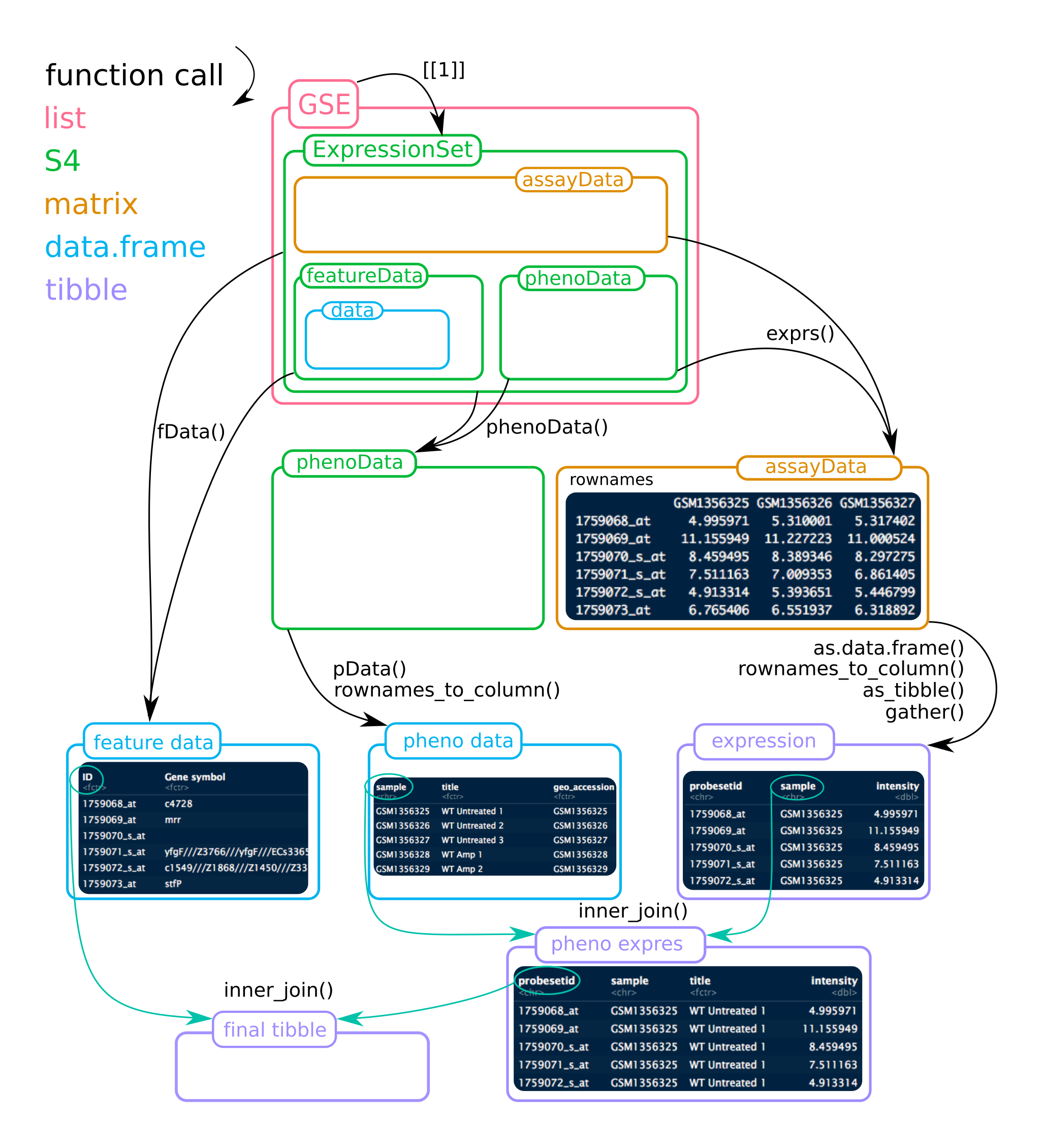
• Two platforms were used in this study, which ones?

• How can you assign the mRNA or mir data to each element of gse35834?

Explore the mRNA expression meta-data

You can use phenoData() to get informations on samples or pData() to retrieve them directly as a data.frame.

• Extract the mRNA meta-data as a tibble which you will name rna_meta
  • rename geo_accession to sample
  • retain only the columns source_name_ch1 and starting with "charact"

Explore the mir expression meta-data

• Extract the mir meta-data as a tibble which you will name mir_meta
  • rename geo_accession to sample
  • retain only the columns source_name_ch1 and all starting with “charact”

Join the meta-data

• Explore the two data frames with View(rna_meta) and View(mir_meta). Are the samples GSM* identical?

We would like to somehow join both informations.
Knowing that both data frames have different sample columns, merge them to get the correspondence between RNA GSM* and mir GSM*. Save the result as rna_mir.

Get RNA expression data for the ENTPD5 gene

Expression data can be accessed using exprs() which returns a matrix.

exprs(gse35834[[1]]) %>% head()

• rows are probes and columns are sample ids in the form of GSM*.
• Probe ids by themselves are not meaningful, but fData() provides features.

fData(gse35834[[1]]) %>% head()

Again, we need to merge both informations to assign the expression data to the gene of interest.

1. Find the common values that that allow us to join both data frames.

2. The rownames contain the necessary informations. But as a matrix contains, by definition, only a single data type (here numerical values), you will need to transform it to a data.frame and convert the rownames to a column using rownames_to_column(var = "ID").
   Save the result as rna_expression

3. merge the expression data to the platform annotations (fData(gse35834[[1]])). Save the result as rna_expression (Don’t worry: R is always working on temporary objects and you won’t erase the object you are working on).

4. Find the Entrez gene id for ENTPD5. Usually, the gene symbol is given in the annotation, but each GEO submission is a new discovery.

5. Filter rna_expression for the gene of interest (ENTPD5) and tidy the samples:
   A column sample for all GSM* and a column rna_expression containing the expression values. Save the result as rna_expression_melt. At this point you should get a tibble of 80 values.

6. Add the meta-data and discard the columns ID, SPOT_ID and sample_mir. Save the result as rna_expression_melt.

Get mir expression data for miR-182

1. Repeat the previous step but using exprs(gse35834[[2]]) for the mir_expression. This time, the mir names are nicely provided by fData(gse35834[[2]]) in the column miRNA_ID_LIST.

2. How many rows do you obtain? How many are expected?

3. Find out what happened, and plot the boxplot distribution of expression by ID

4. Filter out the irrelevant IDs using grepl in the filter function.

5. Add the meta-data, count the number of rows. Discard the column sample_rna after joining.

join both expression

Join rna_expression_melt and mir_expression_melt by their common columns EXCEPT sample. Save the result as expression.

Examine gene expression according to meta data

1. Plot the gene expression distribution by Gender. Is there any obvious difference?

2. Plot gene AND mir expression distribution by Gender. Is there any obvious difference?

3. Plot gene AND mir expression distributions by source (control / cancer). To make it easier, a quick hack is separate(expression, source_name_ch1, c("source", "rest"), sep = 12) to get source as control / cancer. Is there any difference?

4. Do the same plot as in 3. but reorder the levels so that normal colon appears first. Display normal in “lightgreen” and cancer in “red” using scale_fill_manual().

plot relation ENTPD5 ~ mir-182 as scatter-plot for all patients

• add a linear trend using geom_smooth() for all data + per source

• does it support the claim of the study?

linear models

• get the estimate from the linear trend for each source. linear models are outputted by lm() as lists. Since data.frame are much easier to work with, David Robinson developed broom.

The estimate of the intercept is not meaningful thus it is filtered out. One can easily see that the slope is not significant when data are slipped by source.

• Perform the linear regression and tidy the results for all data, is it significant?

• replace tidy by glance to extract the \(r^2\). Is this value satisfactory?

Perform a linear model for the expression of ENTPD5 and ALL mirs

• Count how many hsa-mir, which are not star, are present on the array GPL8786

• Retrieve the expression values for the 677 human mir like you did before. Same procedure, except that you don’t filter for mir-182. Save as all_mir_rna_expression

• Perform the 677 linear models, tidy the results and arrange by the adj.r.squared

• Get the top 12 mir and plot the scatter plot