Data structures

2 May 2017

Learning objectives

(re)view some R base
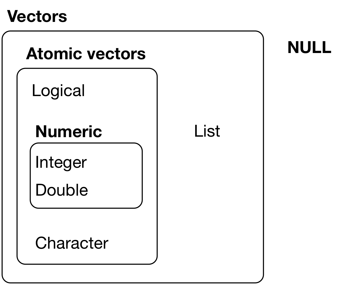
get the different data types: numeric, logical, factor …
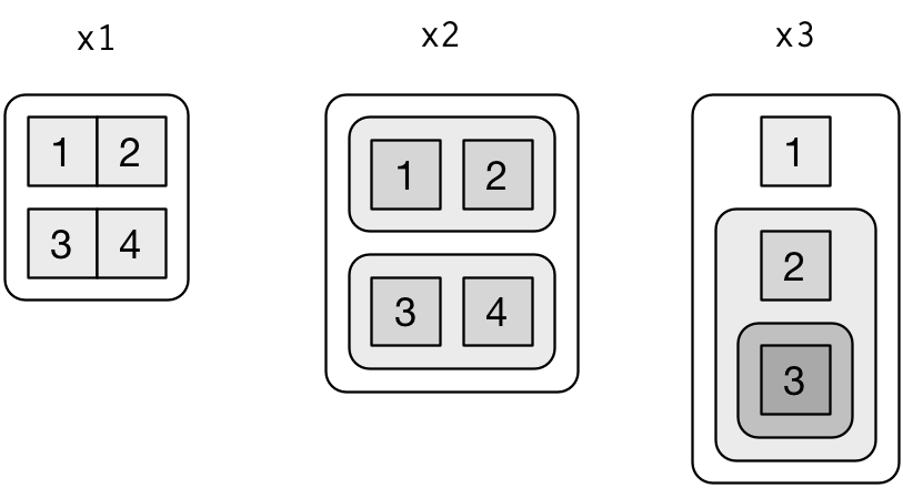
understand what is a list, a vector, a data.frame …

Getting started

Let's get ready to use R and RStudio. Do the following:

Open up RStudio
Maximize the RStudio window
Click the Console pane, at the prompt (>) type in 3 + 2 and hit enter

> 3 + 2

Arithmetic operations

You will not be surprised that R is very good at computing

arithmetic operators

+: addition
-: subtraction
*: multiplication
/: division
^ or **: exponentiation
%%: modulo (remainder after division)
%/%: integer division

Remember

R will:

first perform exponentiation
then multiplications and/or divisions
and finally additions and/or subtractions.

If you need to change the priority during the evaluation, use parentheses – i.e. ( and ) – to group calculations.

Data types and structures

R base

Necessary R base

R base

We could let base down, but the tidyverse is wrapping around it. Some functions need to be known

4 main types

Type	Example
numeric	integer (2), double (2.34)
string	"tidyverse !"
boolean	TRUE / FALSE
complex	2+0i

Special case

NA   # not available, missing data
NA_real_
NA_integer_
NA_character_
NA_complex_
NULL # empty
-Inf/Inf # infinite values

missing and infinite

c(NA_real_, 2.45, 45.67)

[1]    NA  2.45 45.67

c(Inf, 2.45, 45.67)

[1]   Inf  2.45 45.67

Structures

Vectors

c() is the function for concatenate

Example

4
c(43, 5.6, 2.90)

[1] 4
[1] 43.0  5.6  2.9

Factors

convert strings to factors, levels is the dictionary

Example

factor(c("AA", "BB", "AA", "CC"))

[1] AA BB AA CC
Levels: AA BB CC

Matrix (2D), Arrays ($\geq$ 3D)

won't dig into those

Example

matrix(1:4, nrow = 2)

     [,1] [,2]
[1,]    1    3
[2,]    2    4

Lists

very important as can contain anything

Example

list(f = factor(c("AA", "AA")),
     v = c(43, 5.6, 2.90),
     s = 4)

$f
[1] AA AA
Levels: AA

$v
[1] 43.0  5.6  2.9

$s
[1] 4

Data frames are special lists

`data.frame`

same as list but where all objects must have the same length

Example

data.frame(
  f = c("AA", "AA", "BB") %>% factor(),
  v = c(43, 5.6, 2.90),
  s = rep(4, 3))

   f    v s
1 AA 43.0 4
2 AA  5.6 4
3 BB  2.9 4

Data types 2

# evaluate
typeof(2)

[1] "double"

# check
is.integer(2.34)

[1] FALSE

# check with an actual integer
is.integer(2L)

[1] TRUE

# convert
as.integer(2.34)

[1] 2

Vectors

Vectors are the simplest type of object in R.

print(5)

[1] 5

[1] means we made a numeric vector of length 1. Now look at what the : operator does:

1:30

 [1]  1  2  3  4  5  6  7  8  9 10 11 12 13 14 15 16 17 18 19 20 21 22 23
[24] 24 25 26 27 28 29 30

How many elements are in the thing we made here? What does the [24] signify?

Vectors

concatenate

Think of vectors as collections of simple things (like numbers) that are ordered. We can create vectors from other vectors using the c function:

c(2, TRUE, "a string")

[1] "2"        "TRUE"     "a string"

We can use the assignment operator <- to associate a name to our vectors in order to reuse them:

my_vec <- c(3, 4, 1:3)
my_vec

[1] 3 4 1 2 3

Tip

Rstudio has the built-in shortcut Alt+- for <-

Advice

Even if = works also for <-, don't use it, see why

Vectors

(cont.)

The following will build a character vector. We know this because the elements are all in "quotes".

char_vec <- c("dog", "cat", "ape")

Now use the c function to combine a length-one vector number of the number 4 with the char_vec. What happens?

c(4, char_vec)

[1] "4"   "dog" "cat" "ape"

Notice that the 4 is quoted. R turned it into a character vector and then combined it with char_vec.

Remember

All elements in a atomic vector must be of the same type. Otherwise, they are silently coerced.

Vectors

Hierachy

source: H. Wickham - R for data science, licence CC

Vectors

built-in

R has a few built in vectors. One of these is LETTERS. What does it contain?

LETTERS

 [1] "A" "B" "C" "D" "E" "F" "G" "H" "I" "J" "K" "L" "M" "N" "O" "P" "Q"
[18] "R" "S" "T" "U" "V" "W" "X" "Y" "Z"

How do extract the first element from this (the letter A). Here is how to do it:

LETTERS[1]

[1] "A"

Use the square brackets [] to subset vectors

Vectors

subset

Important

Unlike python or Perl, vectors use 1-based index!!

How to extract > 1 element

select elements from position 3 to 10:

LETTERS[3:10]

[1] "C" "D" "E" "F" "G" "H" "I" "J"

Remember what the `:` operator does?

Take a look:

3:10

[1]  3  4  5  6  7  8  9 10

Can you see how LETTERS[3:10] works now?

Exercise

find a way to output

[1] "B" "C" "D" "E"

find a way to output

[1] "B" "C" "D" "E" "G"

find a way to output first 5 letters + one to the last

[1] "A" "B" "C" "D" "E" "Y"

Tip

the length of a vector is provided by length()

find a way to output all letters except the first one

 [1] "B" "C" "D" "E" "F" "G" "H" "I" "J" "K" "L" "M" "N" "O" "P" "Q" "R"
[18] "S" "T" "U" "V" "W" "X" "Y" "Z"

Tip

subsetting could use negative indexes

Solution

indexes from 2 to 5

LETTERS[2:5]

[1] "B" "C" "D" "E"

- indexes from 2 to 5 + 7

LETTERS[c(2:5, 7)]

[1] "B" "C" "D" "E" "G"

- indexes from 1 to 5 + last one

LETTERS[c(1:5, length(LETTERS) - 1)]

[1] "A" "B" "C" "D" "E" "Y"

- indexes except 1

LETTERS[-1]

 [1] "B" "C" "D" "E" "F" "G" "H" "I" "J" "K" "L" "M" "N" "O" "P" "Q" "R"
[18] "S" "T" "U" "V" "W" "X" "Y" "Z"

Named vectors

Like the dict in python or associative array in Perl, characters can be used as indexes

char_vec[1]

[1] "dog"

names(char_vec) <- c("first", "second", "third")
char_vec["first"]

first 
"dog"

Of note, see that the [1] is no longer displayed

char_vec

 first second  third 
 "dog"  "cat"  "ape"

Vectorized operation

my_vec <- 10:18
my_vec + 2

[1] 12 13 14 15 16 17 18 19 20

R recycles vectors that are too short, without any warnings:

my_vec * c(1:3)

[1] 10 22 36 13 28 45 16 34 54

Vectorized operation

(cont.)

Have a look at the following operation:

c(1:3) + c(1:2) * c(1:4)

Warning in c(1:3) + c(1:2) * c(1:4): longer object length is not a multiple
of shorter object length

[1] 2 6 6 9

Details

Steps R performs behind the scene are:

c(1, 2, 3, 1) + (c(1, 2, 1, 2) * c(1, 2, 3, 4))

[1] 2 6 6 9

c(1, 2, 3, 1) + c(1, 4, 3, 8)

[1] 2 6 6 9

Vectors

tricky filling

x <- numeric(10)
x[20] <- 1
head(x, 20)

 [1]  0  0  0  0  0  0  0  0  0  0 NA NA NA NA NA NA NA NA NA  1

source: Kevin Ushey

Warning!

Unlike python that will output index out of range, R expand and fill with missing values silently

Factors

Vectors with qualitative data

my_f <- factor(c("cytoplasm", "nucleus", "extracellular", "nucleus", "nucleus"))
my_f

[1] cytoplasm     nucleus       extracellular nucleus       nucleus      
Levels: cytoplasm extracellular nucleus

Representation

Actually, data are represented with numbers

str(my_f)

 Factor w/ 3 levels "cytoplasm","extracellular",..: 1 3 2 3 3

Dictionary

ids are called levels. Default is alphabetical sorting

levels(my_f)

[1] "cytoplasm"     "extracellular" "nucleus"

For moving around those levels, safest way is to use the forcats package

Matrix

A matrix is a 2D array

M <- matrix(1:6, ncol = 2, nrow = 3)
M

     [,1] [,2]
[1,]    1    4
[2,]    2    5
[3,]    3    6

M <- matrix(1:6, ncol = 2, nrow = 3, byrow = TRUE)
M

     [,1] [,2]
[1,]    1    2
[2,]    3    4
[3,]    5    6

Array

Similar to a matrix but with dimensions $\geq$ 3D

A <- array(1:24, dim = c(2, 4, 3))
A

, , 1

     [,1] [,2] [,3] [,4]
[1,]    1    3    5    7
[2,]    2    4    6    8

, , 2

     [,1] [,2] [,3] [,4]
[1,]    9   11   13   15
[2,]   10   12   14   16

, , 3

     [,1] [,2] [,3] [,4]
[1,]   17   19   21   23
[2,]   18   20   22   24

Lists

Also named recursive vectors. Most permissive type, could contain anything and be nested!

squares are atomic
rounded are lists

source: H. Wickham - R for data science, licence CC

Lists

Pepper analogy

Indexing lists in #rstats. Inspired by the Residence Inn pic.twitter.com/YQ6axb2w7t
— Hadley Wickham (@hadleywickham) 14 septembre 2015

Example

l <- list(name = "Farina",
          firstname = "Geoff",
          year = 1995)

l["firstname"]

$firstname
[1] "Geoff"

l[["firstname"]]

[1] "Geoff"

Question

How to subset a single pepper seed?

Data frames

It's the most important type to recall. All the tidyverse is focusing on those.

Actually on tweaked data.frame: tibbles

definition

data.frame are lists where all columns (i.e vectors) are of the same length

built-in example

women

   height weight
1      58    115
2      59    117
3      60    120
4      61    123
5      62    126
6      63    129
7      64    132
8      65    135
9      66    139
10     67    142
11     68    146
12     69    150
13     70    154
14     71    159
15     72    164

Data frames

subset

We can extract a vector (colum) from a data frame in a few different ways:

Using the double `[[]]`

women[["height"]]

 [1] 58 59 60 61 62 63 64 65 66 67 68 69 70 71 72

Or its alias: the `$` operator

women$height

 [1] 58 59 60 61 62 63 64 65 66 67 68 69 70 71 72

Remember the pepper analogy introduced by Hadley?

What would be the output of women["height"]?

Data frame as a table

A data frame can be considered as a table and extract a specify a cell by its row and column:

first 5 rows

head(women, 5)

  height weight
1     58    115
2     59    117
3     60    120
4     61    123
5     62    126

only one cell with `[]`

first coordinate = row, col]
second coordinate = col

women[4, 2]

[1] 123

Logical operators

In addition to the arithmetic operators

Perform comparisons

== equal
!= different
< smaller
<= smaller or equal
> greater
>= greater or equal
! is not
&, && and
|, || or

Using `library()`

with only `base` loaded

x <- 1:10
filter(x, rep(1, 3))

Time Series:
Start = 1 
End = 10 
Frequency = 1 
 [1] NA  6  9 12 15 18 21 24 27 NA

Conflicts! when 2 packages export a function

with the same name, the latest loaded wins

library(dplyr)
filter(x, rep(1, 3))

Error in UseMethod("filter_") : no applicable method for 'filter_' applied to an object of class "c('integer', 'numeric')

Solution

using the :: operator to call a function from a specific package

stats::filter(x, rep(1, 3))

Time Series:
Start = 1 
End = 10 
Frequency = 1 
 [1] NA  6  9 12 15 18 21 24 27 NA

Pipes with magrittr

developed by Stefan Milton Bache

compare the approaches between classic parenthesis and the magrittr pipeline

R base

set.seed(12)
round(mean(rnorm(5)), 2)

[1] -0.76

magrittr

set.seed(12)
rnorm(5) %>%
  mean() %>%
  round(2)

[1] -0.76

Of note, magrittr needs to loaded with either:

library(magrittr)
library(dplyr)
library(tidyverse)

Coding's style

R is rather flexible and permissive with its syntax. However, being more strict tends to ease the debugging process.

See tidyverse style's recommendations

In summary:

Good

use spaces
use more lines
- } alone on their line except for
r } else {
- using the pipe %>% to display a single instruction per line
- break list definitions, function arguments …
avoid using names of existing functions and variables
use snake_case more than CamelCases

Bad

# example from http://adv-r.had.co.nz/Style.html
T <- FALSE
c <- 10
mean <- function(x) sum(x)

# lack spaces for readibility
average<-mean(feet/12+inches,na.rm=TRUE)

Learning objectives

Getting started

Arithmetic operations

arithmetic operators

Remember

Data types and structures

R base

Necessary R base

R base

4 main types

Special case

missing and infinite

Structures

Vectors

Example

Factors

Example

Matrix (2D), Arrays (\(\geq\) 3D)

Example

Lists

Example

Data frames are special lists

data.frame

Example

Data types 2

Vectors

Vectors

Vectors

concatenate

Tip

Advice

Vectors

(cont.)

Remember

Vectors

Hierachy

Vectors

built-in

Vectors

subset

Important

How to extract > 1 element

Remember what the : operator does?

Exercise

find a way to output

find a way to output

find a way to output first 5 letters + one to the last

Tip

find a way to output all letters except the first one

Tip

Solution

Named vectors

Vectorized operation

Vectorized operation

(cont.)

Details

Vectors

tricky filling

Warning!

Factors

Representation

Dictionary

Matrix

Array

Lists

Lists

Pepper analogy

Example

Question

Data frames

definition

built-in example

Data frames

subset

Using the double [[]]

Or its alias: the $ operator

Remember the pepper analogy introduced by Hadley?

Data frame as a table

first 5 rows

only one cell with []

`data.frame`

Remember what the `:` operator does?

Using the double `[[]]`

Or its alias: the `$` operator

only one cell with `[]`

Using `library()`

with only `base` loaded