Importing data

2 May 2017

Learning objectives

You will learn to:

use readr and/or readxl to import your data into R
use the interactive RStudio interface to visualise your data
appreciate tibbles
adjust the type of the data you would like to import

Importing data

Represents probably the first step of your work
R can handle multiple data types
- flat files (.csv, .tsv, …)
- excel files (.xls, .xlsx)
- foreign statistical formats (.sas from SAS, .sav from SPSS, .dta from Stata)
- databases (SQL, SQLite …)

Tidyverse implementation

R base already provides functions for text files (i.e. read.csv(), read.delim())
tidyverse redefines these functions:
- speed
- characters are not coerced to factors by default
- generates tibbles

Tibbles

have a refined print method that shows only the first 10 rows.
show all the columns that fit on screen and list the name of remaining ones.
each column reports its type.
makes it much easier to work with large data.

Hint

Use as_tibble() to convert a data.frame to a tibble

Tibbles

`tibble` vs `data.frame`

`data.frame`

iris

    Sepal.Length Sepal.Width Petal.Length Petal.Width    Species
1            5.1         3.5          1.4         0.2     setosa
2            4.9         3.0          1.4         0.2     setosa
3            4.7         3.2          1.3         0.2     setosa
4            4.6         3.1          1.5         0.2     setosa
5            5.0         3.6          1.4         0.2     setosa
6            5.4         3.9          1.7         0.4     setosa
7            4.6         3.4          1.4         0.3     setosa
8            5.0         3.4          1.5         0.2     setosa
9            4.4         2.9          1.4         0.2     setosa
10           4.9         3.1          1.5         0.1     setosa
11           5.4         3.7          1.5         0.2     setosa
12           4.8         3.4          1.6         0.2     setosa
13           4.8         3.0          1.4         0.1     setosa
14           4.3         3.0          1.1         0.1     setosa
15           5.8         4.0          1.2         0.2     setosa
16           5.7         4.4          1.5         0.4     setosa
17           5.4         3.9          1.3         0.4     setosa
18           5.1         3.5          1.4         0.3     setosa
19           5.7         3.8          1.7         0.3     setosa
20           5.1         3.8          1.5         0.3     setosa
21           5.4         3.4          1.7         0.2     setosa
22           5.1         3.7          1.5         0.4     setosa
23           4.6         3.6          1.0         0.2     setosa
24           5.1         3.3          1.7         0.5     setosa
25           4.8         3.4          1.9         0.2     setosa
26           5.0         3.0          1.6         0.2     setosa
27           5.0         3.4          1.6         0.4     setosa
28           5.2         3.5          1.5         0.2     setosa
29           5.2         3.4          1.4         0.2     setosa
30           4.7         3.2          1.6         0.2     setosa
31           4.8         3.1          1.6         0.2     setosa
32           5.4         3.4          1.5         0.4     setosa
33           5.2         4.1          1.5         0.1     setosa
34           5.5         4.2          1.4         0.2     setosa
35           4.9         3.1          1.5         0.2     setosa
36           5.0         3.2          1.2         0.2     setosa
37           5.5         3.5          1.3         0.2     setosa
38           4.9         3.6          1.4         0.1     setosa
39           4.4         3.0          1.3         0.2     setosa
40           5.1         3.4          1.5         0.2     setosa
41           5.0         3.5          1.3         0.3     setosa
42           4.5         2.3          1.3         0.3     setosa
43           4.4         3.2          1.3         0.2     setosa
44           5.0         3.5          1.6         0.6     setosa
45           5.1         3.8          1.9         0.4     setosa
46           4.8         3.0          1.4         0.3     setosa
47           5.1         3.8          1.6         0.2     setosa
48           4.6         3.2          1.4         0.2     setosa
49           5.3         3.7          1.5         0.2     setosa
50           5.0         3.3          1.4         0.2     setosa
51           7.0         3.2          4.7         1.4 versicolor
52           6.4         3.2          4.5         1.5 versicolor
53           6.9         3.1          4.9         1.5 versicolor
54           5.5         2.3          4.0         1.3 versicolor
55           6.5         2.8          4.6         1.5 versicolor
56           5.7         2.8          4.5         1.3 versicolor
57           6.3         3.3          4.7         1.6 versicolor
58           4.9         2.4          3.3         1.0 versicolor
59           6.6         2.9          4.6         1.3 versicolor
60           5.2         2.7          3.9         1.4 versicolor
61           5.0         2.0          3.5         1.0 versicolor
62           5.9         3.0          4.2         1.5 versicolor
63           6.0         2.2          4.0         1.0 versicolor
64           6.1         2.9          4.7         1.4 versicolor
65           5.6         2.9          3.6         1.3 versicolor
66           6.7         3.1          4.4         1.4 versicolor
67           5.6         3.0          4.5         1.5 versicolor
68           5.8         2.7          4.1         1.0 versicolor
69           6.2         2.2          4.5         1.5 versicolor
70           5.6         2.5          3.9         1.1 versicolor
71           5.9         3.2          4.8         1.8 versicolor
72           6.1         2.8          4.0         1.3 versicolor
73           6.3         2.5          4.9         1.5 versicolor
74           6.1         2.8          4.7         1.2 versicolor
75           6.4         2.9          4.3         1.3 versicolor
76           6.6         3.0          4.4         1.4 versicolor
77           6.8         2.8          4.8         1.4 versicolor
78           6.7         3.0          5.0         1.7 versicolor
79           6.0         2.9          4.5         1.5 versicolor
80           5.7         2.6          3.5         1.0 versicolor
81           5.5         2.4          3.8         1.1 versicolor
82           5.5         2.4          3.7         1.0 versicolor
83           5.8         2.7          3.9         1.2 versicolor
84           6.0         2.7          5.1         1.6 versicolor
85           5.4         3.0          4.5         1.5 versicolor
86           6.0         3.4          4.5         1.6 versicolor
87           6.7         3.1          4.7         1.5 versicolor
88           6.3         2.3          4.4         1.3 versicolor
89           5.6         3.0          4.1         1.3 versicolor
90           5.5         2.5          4.0         1.3 versicolor
91           5.5         2.6          4.4         1.2 versicolor
92           6.1         3.0          4.6         1.4 versicolor
93           5.8         2.6          4.0         1.2 versicolor
94           5.0         2.3          3.3         1.0 versicolor
95           5.6         2.7          4.2         1.3 versicolor
96           5.7         3.0          4.2         1.2 versicolor
97           5.7         2.9          4.2         1.3 versicolor
98           6.2         2.9          4.3         1.3 versicolor
99           5.1         2.5          3.0         1.1 versicolor
100          5.7         2.8          4.1         1.3 versicolor
101          6.3         3.3          6.0         2.5  virginica
102          5.8         2.7          5.1         1.9  virginica
103          7.1         3.0          5.9         2.1  virginica
104          6.3         2.9          5.6         1.8  virginica
105          6.5         3.0          5.8         2.2  virginica
106          7.6         3.0          6.6         2.1  virginica
107          4.9         2.5          4.5         1.7  virginica
108          7.3         2.9          6.3         1.8  virginica
109          6.7         2.5          5.8         1.8  virginica
110          7.2         3.6          6.1         2.5  virginica
111          6.5         3.2          5.1         2.0  virginica
112          6.4         2.7          5.3         1.9  virginica
113          6.8         3.0          5.5         2.1  virginica
114          5.7         2.5          5.0         2.0  virginica
115          5.8         2.8          5.1         2.4  virginica
116          6.4         3.2          5.3         2.3  virginica
117          6.5         3.0          5.5         1.8  virginica
118          7.7         3.8          6.7         2.2  virginica
119          7.7         2.6          6.9         2.3  virginica
120          6.0         2.2          5.0         1.5  virginica
121          6.9         3.2          5.7         2.3  virginica
122          5.6         2.8          4.9         2.0  virginica
123          7.7         2.8          6.7         2.0  virginica
124          6.3         2.7          4.9         1.8  virginica
125          6.7         3.3          5.7         2.1  virginica
126          7.2         3.2          6.0         1.8  virginica
127          6.2         2.8          4.8         1.8  virginica
128          6.1         3.0          4.9         1.8  virginica
129          6.4         2.8          5.6         2.1  virginica
130          7.2         3.0          5.8         1.6  virginica
131          7.4         2.8          6.1         1.9  virginica
132          7.9         3.8          6.4         2.0  virginica
133          6.4         2.8          5.6         2.2  virginica
134          6.3         2.8          5.1         1.5  virginica
135          6.1         2.6          5.6         1.4  virginica
136          7.7         3.0          6.1         2.3  virginica
137          6.3         3.4          5.6         2.4  virginica
138          6.4         3.1          5.5         1.8  virginica
139          6.0         3.0          4.8         1.8  virginica
140          6.9         3.1          5.4         2.1  virginica
141          6.7         3.1          5.6         2.4  virginica
142          6.9         3.1          5.1         2.3  virginica
143          5.8         2.7          5.1         1.9  virginica
144          6.8         3.2          5.9         2.3  virginica
145          6.7         3.3          5.7         2.5  virginica
146          6.7         3.0          5.2         2.3  virginica
147          6.3         2.5          5.0         1.9  virginica
148          6.5         3.0          5.2         2.0  virginica
149          6.2         3.4          5.4         2.3  virginica
150          5.9         3.0          5.1         1.8  virginica

Tibbles

`tibble` vs `data.frame`

`tibble`

iris %>% as_tibble()

# A tibble: 150 x 5
   Sepal.Length Sepal.Width Petal.Length Petal.Width Species
          <dbl>       <dbl>        <dbl>       <dbl>  <fctr>
 1          5.1         3.5          1.4         0.2  setosa
 2          4.9         3.0          1.4         0.2  setosa
 3          4.7         3.2          1.3         0.2  setosa
 4          4.6         3.1          1.5         0.2  setosa
 5          5.0         3.6          1.4         0.2  setosa
 6          5.4         3.9          1.7         0.4  setosa
 7          4.6         3.4          1.4         0.3  setosa
 8          5.0         3.4          1.5         0.2  setosa
 9          4.4         2.9          1.4         0.2  setosa
10          4.9         3.1          1.5         0.1  setosa
# ... with 140 more rows

`tibble` adjusts to width

iris %>% as_tibble()

# A tibble: 150 x 5
   Sepal.Length Sepal.Width
          <dbl>       <dbl>
 1          5.1         3.5
 2          4.9         3.0
 3          4.7         3.2
 4          4.6         3.1
 5          5.0         3.6
 6          5.4         3.9
 7          4.6         3.4
 8          5.0         3.4
 9          4.4         2.9
10          4.9         3.1
# ... with 140 more rows, and
#   3 more variables:
#   Petal.Length <dbl>,
#   Petal.Width <dbl>,
#   Species <fctr>

tibble printing enhancements

column type is visible
shows only the first 10 rows
shows only the columns that fit on the screen

Create tibbles

`tibble()`

similar to base::data.frame() but
- does not coerce characters to factors
- does not change column names
- never uses rownames

data.frame(`bad name` = 1:4,
           x = rep(letters[1:2], 2)) %>%
  str()

'data.frame':   4 obs. of  2 variables:
 $ bad.name: int  1 2 3 4
 $ x       : Factor w/ 2 levels "a","b": 1 2 1 2

tibble(`bad name` = 1:4,
       x = rep(letters[1:2], 2)) %>%
  str()

Classes 'tbl_df', 'tbl' and 'data.frame':   4 obs. of  2 variables:
 $ bad name: int  1 2 3 4
 $ x       : chr  "a" "b" "a" "b"

`tribble()`

transposed tibble
row-by-row layout
columns are defined by formula (~)

tribble(
  ~x, ~y,  ~z,
  "a", 2,  3.6,
  "b", 1,  8.5
)

# A tibble: 2 x 3
      x     y     z
  <chr> <dbl> <dbl>
1     a     2   3.6
2     b     1   8.5

Create tibbles

Create tibbles by copy paste

datapasta package
can be useful to copy paste small datasets
Rstudio addin
have a look at the vignette

The tidyverse packages to import your data

Tidyverse packages to import your data

Seven file formats are supported by the readr package:

read_csv(): comma separated (CSV) files
read_tsv(): tab separated files
read_delim(): general delimited files
read_fwf(): fixed width files
read_table(): tabular files where colums are separated by white-space.
read_log(): web log files

readxl

To import excel files (.xls and .xlsx):

read_excel()
- read_xls()
- read_xlsx()

haven

read_sas() for SAS
read_sav() for SPSS
read_dta() for Stata

Rstudio data import

interactive call to `readr` or `readxl`

Import button

Use the Import Dataset button in the upper right panel or click on the file in the lower right panel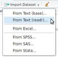

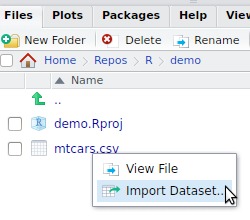
Will interactively select the appropriate function
Copy paste the generated command to your Rmarkdown document

Example

Create a new project (easier to setup the root project path)
Run the following command to copy the mtcars.csv file shipped with readr to your project folder:

file.copy(
  from = readr::readr_example("mtcars.csv"),
  to = "mtcars.csv"
  )

Use the interactive Import Dataset button to import the mtcars.csv file.

Rstudio data import

preview window

Importing flat files

`readr` functions

`read_csv()`

Comma delimited files

`read_csv2()`

Semi-colon delimited files

`read_tsv()`

tab delimited files

`read_delim()`

any delimiter:

read_delim(file, delim = "|", ...)

`read_fwf()`

fixed width files

Reading flat files

csv file

Example of `csv` file: mtcars.csv

"mpg","cyl","disp","hp","drat","wt","qsec","vs","am","gear","carb"
21,6,160,110,3.9,2.62,16.46,0,1,4,4
21,6,160,110,3.9,2.875,17.02,0,1,4,4
22.8,4,108,93,3.85,2.32,18.61,1,1,4,1
21.4,6,258,110,3.08,3.215,19.44,1,0,3,1
18.7,8,360,175,3.15,3.44,17.02,0,0,3,2
...

Using `read_csv()`

readr provides some example files
use readr::readr_example() to access them
is able to read local and remote files
is able to read compressed files (.zip, .gz, …)

Reading flat files

csv file

Using `read_csv()`

readr_example("mtcars.csv") %>% # Generates the path to the example file
  read_csv()

Parsed with column specification:
cols(
  mpg = col_double(),
  cyl = col_integer(),
  disp = col_double(),
  hp = col_integer(),
  drat = col_double(),
  wt = col_double(),
  qsec = col_double(),
  vs = col_integer(),
  am = col_integer(),
  gear = col_integer(),
  carb = col_integer()
)

# A tibble: 32 x 11
     mpg   cyl  disp    hp  drat    wt  qsec    vs    am  gear  carb
   <dbl> <int> <dbl> <int> <dbl> <dbl> <dbl> <int> <int> <int> <int>
 1  21.0     6 160.0   110  3.90 2.620 16.46     0     1     4     4
 2  21.0     6 160.0   110  3.90 2.875 17.02     0     1     4     4
 3  22.8     4 108.0    93  3.85 2.320 18.61     1     1     4     1
 4  21.4     6 258.0   110  3.08 3.215 19.44     1     0     3     1
 5  18.7     8 360.0   175  3.15 3.440 17.02     0     0     3     2
 6  18.1     6 225.0   105  2.76 3.460 20.22     1     0     3     1
 7  14.3     8 360.0   245  3.21 3.570 15.84     0     0     3     4
 8  24.4     4 146.7    62  3.69 3.190 20.00     1     0     4     2
 9  22.8     4 140.8    95  3.92 3.150 22.90     1     0     4     2
10  19.2     6 167.6   123  3.92 3.440 18.30     1     0     4     4
# ... with 22 more rows

Reading flat files

csv file

Column types

are guessed from the 1000 first rows
- adjustable guess_max option
guessed types are displayed as a message
to hide this message:
- lazy method 1: set message = FALSE in your rmarkdown chunk option.
- lazy method 2: set col_types = cols()
- Hadley Wickham recommends to adjust the col_types to avoid any problem

Message

Parsed with column specification:
cols(
  mpg = col_double(),
  cyl = col_integer(),
  disp = col_double(),
  hp = col_integer(),
  drat = col_double(),
  wt = col_double(),
  qsec = col_double(),
  vs = col_integer(),
  am = col_integer(),
  gear = col_integer(),
  carb = col_integer()
)

Reading flat files

csv file

Explicit method

Use the following functions in cols():

col_double()
col_integer()
col_character()
col_logical()
col_factor()
col_date()
col_datetime()
col_time()
col_guess()
col_skip()

Example 1

readr_example("mtcars.csv") %>%
  read_csv(col_types = cols(mpg = col_double(),
                            cyl = col_integer(),
                            disp = col_double(),
                            hp = col_integer(),
                            drat = col_double(),
                            wt = col_double(),
                            qsec = col_double(),
                            vs = col_integer(),
                            am = col_integer(),
                            gear = col_integer(),
                            carb = col_integer())
  )

Compact string shortcuts

c = character
i = integer
n = number
d = double
l = logical
D = date
T = date time
t = time
? = guess
_/- = skip

Example 2

readr_example("mtcars.csv") %>%
  read_csv(col_types = cols(
    mpg = "d", cyl = "i", disp = "d",
    hp = "i", drat = "d", wt = "d",
    qsec = "d", vs = "i", am = "i",
    gear = "i", carb = "i"))

readr_example("mtcars.csv") %>%
  read_csv(col_types = "dididddiiii")

Try it yourself

Exercise 1

import the mtcars.csv file again but
- read in the number of cylinders as characters.
- skip all columns except miles per gallon, cylinder and the number of gears

Answer

readr_example("mtcars.csv") %>%
  read_csv(col_types = cols_only(cyl = col_character(),
                                 mpg = col_double(),
                                 gear = col_integer()))

# A tibble: 32 x 3
    mpg   cyl  gear
  <dbl> <chr> <int>
1  21.0     6     4
2  21.0     6     4
3  22.8     4     4
4  21.4     6     3
# ... with 28 more rows

readr_example("mtcars.csv") %>%
  read_csv(col_types = "dc_______i_")

# A tibble: 32 x 3
    mpg   cyl  gear
  <dbl> <chr> <int>
1  21.0     6     4
2  21.0     6     4
3  22.8     4     4
4  21.4     6     3
# ... with 28 more rows

Try it yourself

Exercise 2

try to load the file challenge.csv (provided by readr_example())
store the content in an object challenge

Step 1

what happened?
you can use problems(challenge) to list the failures again

challenge <- readr_example("challenge.csv") %>% 
  read_csv()

Parsed with column specification:
cols(
  x = col_integer(),
  y = col_character()
)

Warning in rbind(names(probs), probs_f): number of columns of result is not
a multiple of vector length (arg 1)

Warning: 1000 parsing failures.
row # A tibble: 5 x 5 col     row   col               expected             actual            file expected   <int> <chr>                  <chr>              <chr>           <chr> actual 1  1001     x no trailing characters .23837975086644292 'challenge.csv' file 2  1002     x no trailing characters .41167997173033655 'challenge.csv' row 3  1003     x no trailing characters  .7460716762579978 'challenge.csv' col 4  1004     x no trailing characters   .723450553836301 'challenge.csv' expected 5  1005     x no trailing characters   .614524137461558 'challenge.csv'
... ................. ... ....................................................................... ........ ....................................................................... ...... ....................................................................... .... ....................................................................... ... ....................................................................... ... ....................................................................... ........ .......................................................................
See problems(...) for more details.

Try it yourself

Exercise 2

try to load the file challenge.csv (provided by readr_example())
store the content in an object challenge
override the guessed column type to allow the import

Step 2

method 1

challenge <- readr_example("challenge.csv") %>% 
  read_csv(col_types = "dD")

method 2 (not recommended)

challenge <- readr_example("challenge.csv") %>% 
  read_csv(guess_max = 1500) # n > 1000: look at the first row causing a failure

Parsed with column specification:
cols(
  x = col_double(),
  y = col_date(format = "")
)

Skipping lines

`skip` argument

To skip the first n rows

`n_max` argument

To stop reading after n rows

`col_names` argument

override column names

readr_example("mtcars.csv") %>%
  read_csv()

# A tibble: 32 x 11
    mpg   cyl  disp    hp  drat    wt  qsec    vs    am  gear  carb
  <dbl> <int> <dbl> <int> <dbl> <dbl> <dbl> <int> <int> <int> <int>
1  21.0     6   160   110  3.90 2.620 16.46     0     1     4     4
2  21.0     6   160   110  3.90 2.875 17.02     0     1     4     4
3  22.8     4   108    93  3.85 2.320 18.61     1     1     4     1
4  21.4     6   258   110  3.08 3.215 19.44     1     0     3     1
# ... with 28 more rows

readr_example("mtcars.csv") %>%
  read_csv(skip = 3,
           n_max = 3,
           col_names = FALSE)

# A tibble: 3 x 11
     X1    X2    X3    X4    X5    X6    X7    X8    X9   X10   X11
  <dbl> <int> <int> <int> <dbl> <dbl> <dbl> <int> <int> <int> <int>
1  22.8     4   108    93  3.85 2.320 18.61     1     1     4     1
2  21.4     6   258   110  3.08 3.215 19.44     1     0     3     1
3  18.7     8   360   175  3.15 3.440 17.02     0     0     3     2

readr_example("mtcars.csv") %>%
  read_csv(skip = 3, n_max = 3,
           col_names = c("mpg", "cyl", "disp", "hp", "drat", "wt", "qsec", "vs", "am", "gear", "carb"))

# A tibble: 3 x 11
    mpg   cyl  disp    hp  drat    wt  qsec    vs    am  gear  carb
  <dbl> <int> <int> <int> <dbl> <dbl> <dbl> <int> <int> <int> <int>
1  22.8     4   108    93  3.85 2.320 18.61     1     1     4     1
2  21.4     6   258   110  3.08 3.215 19.44     1     0     3     1
3  18.7     8   360   175  3.15 3.440 17.02     0     0     3     2

Internationalisation

locales

Example

"name";"first_name";"born";"value"
"Dupont";"Michel";03/10/71;1,2
"Doe";"John";27/02/74;1,7
"Mustermann";"Max";14/08/69;1,6

Link to the file: https://git.io/v9Wmf
Trying to import using read_delim()

read_delim("data/locale_1.csv",
           delim = ";")

# A tibble: 3 x 4
        name first_name     born value
       <chr>      <chr>    <chr> <dbl>
1     Dupont     Michel 03/10/71    12
2        Doe       John 27/02/74    17
3 Mustermann        Max 14/08/69    16

dates are detected as characters (minor issue)
decimal numbers are not detected as they should (major issue)

Adjusting the `locale` argument

read_delim("data/locale_1.csv",
           delim = ";",
           locale = locale(decimal_mark = ",",
                           date_format = "%d/%m/%y"))

# A tibble: 3 x 4
        name first_name       born value
       <chr>      <chr>     <date> <dbl>
1     Dupont     Michel 1971-10-03   1.2
2        Doe       John 1974-02-27   1.7
3 Mustermann        Max 1969-08-14   1.6

have a look at ?parse_datetime to list the datetime format specifications
read_csv2() is a shortcut to read_delim() using ; as a delimiter and , as the decimal mark
you still need to adjust the date parsing

read_csv2("data/locale_1.csv",
          locale = locale(date_format = "%d/%m/%y"))

read_csv2("data/locale_1.csv") %>%
  mutate_at(c("born"), parse_date, format = "%d/%m/%y")

Importing MS Excel files

`readxl`

reading MS Excel files

readxl

able to import .xls and .xlsx files
read_excel()
- read_xls()
- read_xlsx()
excel_sheets() to list all sheets in the Excel file

new feature

Version 1.0.0 is out
import cell ranges

Try it yourself

excel file

Sample files

we will use the files shipped with the readxl package
list of available examples:

readxl::readxl_example()

 [1] "clippy.xls"    "clippy.xlsx"   "datasets.xls" 
 [4] "datasets.xlsx" "deaths.xls"    "deaths.xlsx"  
 [7] "geometry.xls"  "geometry.xlsx" "type-me.xls"  
[10] "type-me.xlsx"

Sample files

to get used to readxl and the import of excel files
- use the datasets.xlsx example file
- determine how many sheets are contained in the file
- load the data contained in the mtcars sheet
- you can also try Rstudio's interactive importer
```
file.copy(
  from = readxl::readxl_example("datasets.xlsx"),
  to = "datasets.xlsx"
) # To copy it to the root of your project
```

Try it yourself

excel file

the `deaths` dataset

use the deaths.xls file (using readxl_example("deaths.xlsx") to get the path to it)
how many sheets does the file contain?
import the first sheet of the file.
are you happy with the result?

readxl_example("deaths.xlsx") %>%
  read_excel(sheet = 1)

# A tibble: 18 x 6
              `Lots of people`       X__1  X__2     X__3          X__4
                         <chr>      <chr> <chr>    <chr>         <chr>
1 simply cannot resist writing       <NA>  <NA>     <NA>          <NA>
2                           at        the   top     <NA>            of
3                           or    merging  <NA>     <NA>          <NA>
4                         Name Profession   Age Has kids Date of birth
5                  David Bowie   musician    69     TRUE         17175
6                Carrie Fisher      actor    60     TRUE         20749
7                  Chuck Berry   musician    90     TRUE          9788
8                  Bill Paxton      actor    61     TRUE         20226
# ... with 10 more rows, and 1 more variables: X__5 <chr>

Try it yourself

excel file

Use the new possibilities of readxl 1.0.0 to read in your data frame of interest (have a look at ?readxl::read_excel)

Try it yourself

excel file

readxl_example("deaths.xlsx") %>%
  read_excel(sheet = 1, range = "A5:F15")

# A tibble: 10 x 6
                 Name Profession   Age `Has kids` `Date of birth`
                <chr>      <chr> <dbl>      <lgl>          <dttm>
 1        David Bowie   musician    69       TRUE      1947-01-08
 2      Carrie Fisher      actor    60       TRUE      1956-10-21
 3        Chuck Berry   musician    90       TRUE      1926-10-18
 4        Bill Paxton      actor    61       TRUE      1955-05-17
 5             Prince   musician    57       TRUE      1958-06-07
 6       Alan Rickman      actor    69      FALSE      1946-02-21
 7 Florence Henderson      actor    82       TRUE      1934-02-14
 8         Harper Lee     author    89      FALSE      1926-04-28
 9      Zsa Zsa Gábor      actor    99       TRUE      1917-02-06
10     George Michael   musician    53      FALSE      1963-06-25
# ... with 1 more variables: `Date of death` <dttm>

Alternative calls

readxl_example("deaths.xlsx") %>%
  read_excel(range = "arts!A5:F15")

readxl_example("deaths.xlsx") %>%
  read_excel(range = cell_limits(c(5, 1), c(15, 6), "arts"))
  # have a look at ?cellranger::cell_limits

Reading Excel files

column types

Column types

similar to readr using the col_types argument
but the cols() function won't work here!
- readr guesses column type based on the data.
- readxl guesses column type based on Excel cell types
col_types should be adjusted to a character vector
look at the correspondance in the readxl vignette
```
vignette("cell-and-column-types")
```

How it is in Excel	How it will be in R	How to request in col_types
anything	non-existent	"skip"
empty	logical, but all NA	you cannot request this
boolean	logical	"logical"
numeric	numeric	"numeric"
datetime	POSIXct	"date"
text	character	"text"
anything	list	"list"

Reading Excel files

column types

mixed column types

try to import the clippy.xls example file provided by readxl

readxl_example("clippy.xls") %>% 
  read_excel()

# A tibble: 4 x 2
                  name     value
                 <chr>     <chr>
1                 Name    Clippy
2              Species paperclip
3 Approx date of death     39083
4      Weight in grams       0.9

date of death is coerced to a character
you can override the column type and select one that can handle different types

override `col_types`

readxl_example("clippy.xls") %>% 
  read_excel(col_types = c("text", "list"))

# A tibble: 4 x 2
                  name      value
                 <chr>     <list>
1                 Name  <chr [1]>
2              Species  <chr [1]>
3 Approx date of death <dttm [1]>
4      Weight in grams  <dbl [1]>

readxl_example("clippy.xls") %>% 
  read_excel(col_types = c("text", "list")) %>%
  tibble::deframe() %>%
  str()

List of 4
 $ Name                : chr "Clippy"
 $ Species             : chr "paperclip"
 $ Approx date of death: POSIXct[1:1], format: "2007-01-01"
 $ Weight in grams     : num 0.9

Wrap up

You learned to:

appreciate the tibble printing features
- column types are displayed
use readr and/or readxl to import your data into R
- using the command line
- using the interactive RStudio interface
avoid some common pitfalls during data import
- wrong types
- wrong formats (decimal marks)
adjust the imported data types
select your data of interest in excel files which are often not tidy at all!

Before we stop

Acknowledgments

Hadley Wickham
Jennifer Bryan

Learning objectives

You will learn to:

Importing data

Tidyverse implementation

Tibbles

Tibbles

Hint

Tibbles

tibble vs data.frame

data.frame

Tibbles

tibble vs data.frame

tibble

tibble adjusts to width

tibble printing enhancements

Create tibbles

tibble()

tribble()

Create tibbles

Create tibbles by copy paste

The tidyverse packages to import your data

Tidyverse packages to import your data

readxl

haven

Rstudio data import

interactive call to readr or readxl

Import button

Example

Rstudio data import

preview window

Importing flat files

readr functions

read_csv()

read_csv2()

read_tsv()

read_delim()

read_fwf()

Reading flat files

csv file

Example of csv file: mtcars.csv

Using read_csv()

Reading flat files

csv file

Using read_csv()

Reading flat files

csv file

Column types

Message

Reading flat files

csv file

Explicit method

Example 1

Compact string shortcuts

Example 2

Try it yourself

Exercise 1

Answer

Try it yourself

Exercise 2

Step 1

Try it yourself

Exercise 2

Step 2

Skipping lines

skip argument

n_max argument

col_names argument

Internationalisation

locales

Example

Adjusting the locale argument

Importing MS Excel files

readxl

reading MS Excel files

readxl

new feature

Try it yourself

excel file

Sample files

Sample files

`tibble` vs `data.frame`

`data.frame`

`tibble` vs `data.frame`

`tibble`

`tibble` adjusts to width

`tibble()`

`tribble()`

interactive call to `readr` or `readxl`

`readr` functions

`read_csv()`

`read_csv2()`

`read_tsv()`

`read_delim()`

`read_fwf()`

Example of `csv` file: mtcars.csv

Using `read_csv()`

Using `read_csv()`

`skip` argument

`n_max` argument

`col_names` argument

Adjusting the `locale` argument

`readxl`

the `deaths` dataset

override `col_types`