You will learn to:

- use the markdown syntax
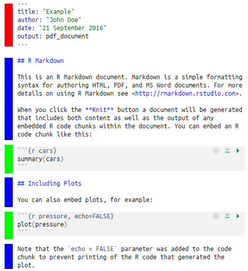
- create Rmarkdown documents
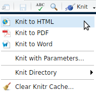
- define the output format you expect to render
- use the interactive RStudio interface to
- create your documents
- insert R code
- build your final document
- use some nice rmarkdown features like
- inserting bibliography
- creating parameterised reports

 +
+