You will learn to:

- use
dplyr/purrrfor efficient data manipulation - tidying linear models using
broom - managing workflow by keeping related things together in one
tibble.
4 May 2017
dplyr / purrr for efficient data manipulationbroomtibble.Tutorial based on the great conference by Hadley Wickham

progress bar will be added


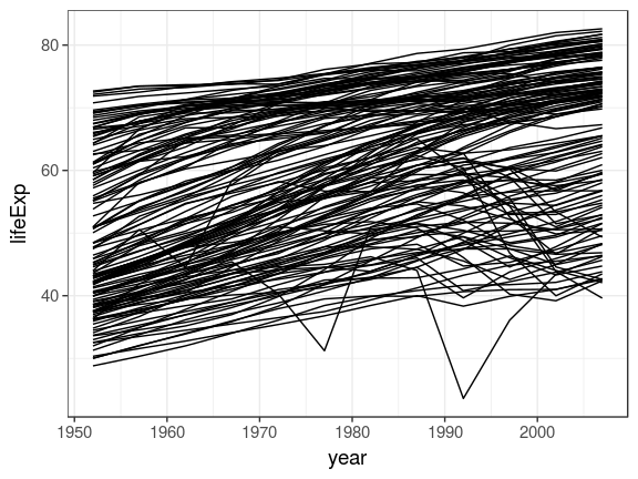
gapminderlibrary("gapminder")
gapminder %>%
ggplot(aes(x = year, y = lifeExp, group = country)) +
geom_line()
by_country <- gapminder %>%
  mutate(year1950 = year - 1950) %>%
  group_by(continent, country) %>%
  nest()
by_country
# A tibble: 142 x 3
   continent     country              data
      <fctr>      <fctr>            <list>
 1      Asia Afghanistan <tibble [12 x 5]>
 2    Europe     Albania <tibble [12 x 5]>
 3    Africa     Algeria <tibble [12 x 5]>
 4    Africa      Angola <tibble [12 x 5]>
 5  Americas   Argentina <tibble [12 x 5]>
 6   Oceania   Australia <tibble [12 x 5]>
 7    Europe     Austria <tibble [12 x 5]>
 8      Asia     Bahrain <tibble [12 x 5]>
 9      Asia  Bangladesh <tibble [12 x 5]>
10    Europe     Belgium <tibble [12 x 5]>
# ... with 132 more rowsyear1950 will help to get count oldest datecontinent to group_by() to keep the infogapminder %>% filter(country == "Germany") %>% select(-country, -continent)
# A tibble: 12 x 4
    year lifeExp      pop gdpPercap
   <int>   <dbl>    <int>     <dbl>
 1  1952  67.500 69145952  7144.114
 2  1957  69.100 71019069 10187.827
 3  1962  70.300 73739117 12902.463
 4  1967  70.800 76368453 14745.626
 5  1972  71.000 78717088 18016.180
 6  1977  72.500 78160773 20512.921
 7  1982  73.800 78335266 22031.533
 8  1987  74.847 77718298 24639.186
 9  1992  76.070 80597764 26505.303
10  1997  77.340 82011073 27788.884
11  2002  78.670 82350671 30035.802
12 2007 79.406 82400996 32170.374by_country %>% filter(country == "Germany") %>% pull(data) # dplyr 0.6, .$data for dplyr 0.5
[[1]]
# A tibble: 12 x 5
    year lifeExp      pop gdpPercap year1950
   <int>   <dbl>    <int>     <dbl>    <dbl>
 1  1952  67.500 69145952  7144.114        2
 2  1957  69.100 71019069 10187.827        7
 3  1962  70.300 73739117 12902.463       12
 4  1967  70.800 76368453 14745.626       17
 5  1972  71.000 78717088 18016.180       22
 6  1977  72.500 78160773 20512.921       27
 7  1982  73.800 78335266 22031.533       32
 8  1987  74.847 77718298 24639.186       37
 9  1992  76.070 80597764 26505.303       42
10  1997  77.340 82011073 27788.884       47
11  2002  78.670 82350671 30035.802       52
12 2007 79.406 82400996 32170.374 57by_country_lm <- by_country %>% mutate(model = map(data, ~ lm(lifeExp ~ year1950, data = .x))) by_country_lm
# A tibble: 142 x 4
   continent     country              data    model
      <fctr>      <fctr>            <list>   <list>
 1      Asia Afghanistan <tibble [12 x 5]> <S3: lm>
 2    Europe     Albania <tibble [12 x 5]> <S3: lm>
 3    Africa     Algeria <tibble [12 x 5]> <S3: lm>
 4    Africa      Angola <tibble [12 x 5]> <S3: lm>
 5  Americas   Argentina <tibble [12 x 5]> <S3: lm>
 6   Oceania   Australia <tibble [12 x 5]> <S3: lm>
 7    Europe     Austria <tibble [12 x 5]> <S3: lm>
 8      Asia     Bahrain <tibble [12 x 5]> <S3: lm>
 9      Asia  Bangladesh <tibble [12 x 5]> <S3: lm>
10    Europe     Belgium <tibble [12 x 5]> <S3: lm>
# ... with 132 more rows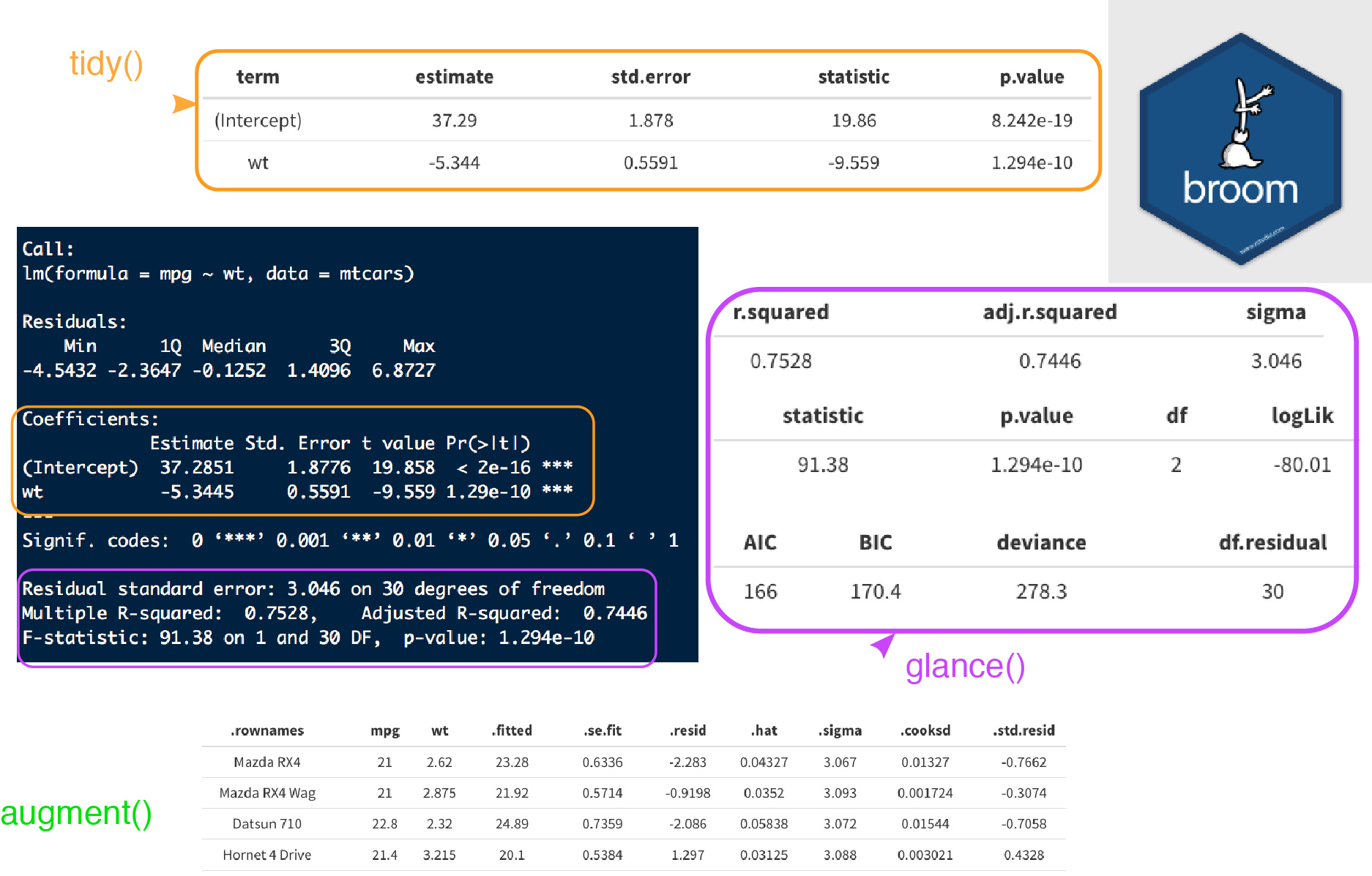
library("broom")
models <- by_country_lm %>%
  mutate(glance  = map(model, glance),
         rsq     = glance %>% map_dbl("r.squared"),
         tidy    = map(model, tidy),
         augment = map(model, augment))
models
# A tibble: 142 x 8
continent country data model glance
<fctr> <fctr> <list> <list> <list>
1 Asia Afghanistan <tibble [12 x 5]> <S3: lm> <data.frame [1 x 11]>
2 Europe Albania <tibble [12 x 5]> <S3: lm> <data.frame [1 x 11]>
3 Africa Algeria <tibble [12 x 5]> <S3: lm> <data.frame [1 x 11]>
4 Africa Angola <tibble [12 x 5]> <S3: lm> <data.frame [1 x 11]>
5 Americas Argentina <tibble [12 x 5]> <S3: lm> <data.frame [1 x 11]>
6 Oceania Australia <tibble [12 x 5]> <S3: lm> <data.frame [1 x 11]>
7 Europe Austria <tibble [12 x 5]> <S3: lm> <data.frame [1 x 11]>
8 Asia Bahrain <tibble [12 x 5]> <S3: lm> <data.frame [1 x 11]>
9 Asia Bangladesh <tibble [12 x 5]> <S3: lm> <data.frame [1 x 11]>
10 Europe Belgium <tibble [12 x 5]> <S3: lm> <data.frame [1 x 11]>
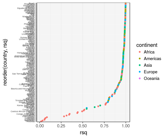
# ... with 132 more rows, and 3 more variables: rsq <dbl>, tidy <list>,
# augment <list>models %>% ggplot(aes(x = rsq, y = reorder(country, rsq))) + geom_point(aes(colour = continent)) + theme(axis.text.y = element_text(size = 6))
models %>%
  filter(rsq < 0.55) %>%
  unnest(data) %>%
  ggplot(aes(x = year, y = lifeExp)) +
  geom_line(aes(colour = continent)) +
  facet_wrap(~ country) +
  theme(legend.justification = c(1, 0),
        legend.position = c(1, 0))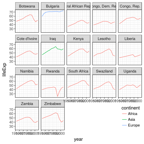
models %>%
  unnest(tidy) %>%
  select(continent, country, rsq, term, estimate) %>%
  spread(term, estimate) %>%
  ggplot(aes(x = `(Intercept)`, y = year1950)) +
  geom_point(aes(colour = continent, size = rsq)) +
  geom_smooth(se = FALSE, method = "loess") +
  scale_size_area() + labs(x = "Life expectancy (1950)", y = "Yearly improvement")

library(gganimate)
gapminder %>%
ggplot(aes(x = gdpPercap,
           y = lifeExp,
           size = pop,
           color = continent,
           frame = year)) +
  geom_point() +
  scale_x_log10() -> p
gganimate(p, 'img/09_gapminder.gif')