This practical work is adapted from the exhaustive example published by David Robinson on his blog.

In 2008, Brauer et al. used microarrays to test the effect of starvation on the growth rate of yeast. For example, they tried limiting the yeast’s supply of glucose (sugar to metabolize into energy), of leucine (an essential amino acid), or of ammonium (a source of nitrogen).

Project - set-up

Create a folder data
Download Brauer2008_DataSet1.tds inside the data folder

Load the [Brauer2008_DataSet1.tds] file as a tibble named original_data. This is the exact data that was published with the paper (though for some reason the link on the journal’s page is broken). It thus serves as a good example of tidying a biological dataset “found in the wild”.

Solution

original_data <- read_tsv("https://lsru.github.io/r_workshop/data/Brauer2008_DataSet1.tds")

## Parsed with column specification:
## cols(
##   .default = col_double(),
##   GID = col_character(),
##   YORF = col_character(),
##   NAME = col_character(),
##   GWEIGHT = col_integer()
## )

## See spec(...) for full column specifications.

1 Tidying the data

Have a look at the dataset. Is the data “tidy”?

Solution

cat(as.character(original_data$NAME[1:3]), sep = "\n")

## SFB2       || ER to Golgi transport || molecular function unknown || YNL049C || 1082129
## || biological process unknown || molecular function unknown || YNL095C || 1086222
## QRI7       || proteolysis and peptidolysis || metalloendopeptidase activity || YDL104C || 1085955

# not tidy at all

1.1 Many variables are stored in one column

Gene name e.g. SFB2. Note that not all genes have a name.
Biological process e.g. “proteolysis and peptidolysis”
Molecular function e.g. “metalloendopeptidase activity”
Systematic ID e.g. YNL049C. Unlike a gene name, every gene in this dataset has a systematic ID.
Another ID number e.g. 1082129. We don’t know what this number means, and it’s not annotated in the paper. Oh, well.

Use the appropriate function provided in the tidyr library to split these values and generate a column for each variable.

Tip

Special characters such as pipes (|) must be despecialized as they have a specific meaning. In R, you have to use 2 backslashes like \\| for one pipe |

Solution

cleaned_data <- original_data %>%
  separate(NAME, c("name", "BP", "MF", "systematic_name", "number"), sep = "\\|\\|")

Once you separated the variables delimited by two “||”, check closer the new values: You will see that they might start and/or end with whitespaces which might be inconvinient during the subsequent use.
- To remove these whitespaces, R base provides a function called trimws(). Let’s test how the function works:
- dplyr allows us to apply a function (in our case trimws()) to all columns. In other words, we would like to modify the content of each column with the output of the function trimws(). How can you achieve this? Save the result in a tibble called cleaned_data.

# Creating test string with whitespaces:
s <- "  Removing whitespaces at both ends "
s

## [1] "  Removing whitespaces at both ends "

trimws(s)

## [1] "Removing whitespaces at both ends"

Solution

cleaned_data <- original_data %>%
  separate(NAME, c("name", "BP", "MF", "systematic_name", "number"), sep = "\\|\\|") %>%
  mutate_at(vars(name:systematic_name), funs(trimws))

We are not going to use every column of the dataframe. Remove the unnecessary columns: number, GID, YORF and GWEIGHT.

Solution

cleaned_data %>%
  select(-number, -GID, -YORF, -GWEIGHT) -> cleaned_data

Look at the column names.
Do you think that our dataset is now “tidy”?

Solution

No, our tibble is still not tidy. We can see that the column names from G0.05 to U0.3 represent a variable.

1.2 Column headers are values, not variable names

Keep care to build a tibble with each column representing a variable: At this point we are storing the sample name (will contain G0.05 …) as a different column sample associated to values in expression column. Save as cleaned_data_melt

Solution

cleaned_data %>%
  gather(sample, expression, G0.05:U0.3) -> cleaned_data_melt

Now look at the content of the sample column. We are again facing the problem that two variables are stored in a single column. The nutrient in the first character, then the growth rate.

Solution

unique(cleaned_data_melt$sample)

##  [1] "G0.05" "G0.1"  "G0.15" "G0.2"  "G0.25" "G0.3"  "N0.05" "N0.1" 
##  [9] "N0.15" "N0.2"  "N0.25" "N0.3"  "P0.05" "P0.1"  "P0.15" "P0.2" 
## [17] "P0.25" "P0.3"  "S0.05" "S0.1"  "S0.15" "S0.2"  "S0.25" "S0.3" 
## [25] "L0.05" "L0.1"  "L0.15" "L0.2"  "L0.25" "L0.3"  "U0.05" "U0.1" 
## [33] "U0.15" "U0.2"  "U0.25" "U0.3"

Use the same function as before to split the sample column into two variables nutrient and rate (use the appropriate delimitation in sep.

Tip

Consider using the convert argument. It allows to convert strings to number when relevant like here.

Solution

cleaned_data_melt %>%
  separate(sample, c("nutrient", "rate"), sep = 1, convert = TRUE) -> cleaned_data_melt

1.3 Turn nutrient letters into more comprehensive words

Right now, the nutrients are designed by a single letter. It would be nice to have the full word instead. One could use a full mixture of if and else such as if_else(nutrient == "G", "Glucose", if_else(nutrient == "L", "Leucine", etc ...)) But, that would be cumbersome.

using the following correspondences and dplyr::recode, recode all nutrient names.

G = "Glucose", L = "Leucine", P = "Phosphate",
S = "Sulfate", N = "Ammonia", U = "Uracil"

Solution

cleaned_data_melt %>%
  mutate(nutrient = recode(nutrient, G = "Glucose", L = "Leucine", P = "Phosphate",
                                     S = "Sulfate", N = "Ammonia", U = "Uracil")) -> cleaned_data_melt

1.4 Cleaning up missing data

Two variables must be present for the further analysis:

gene expression named as expression
systematic id named as systematic_name

delete observations that are missing any of the two mandatory variables. How many rows did you remove?

Solution

cleaned_data_melt %>%
  filter(!is.na(expression), systematic_name != "") -> cleaned_data_melt
# 199,332 - 198,430 = 902 rows deleted

2 Representing the data

Tidying the data is a crucial step allowing easy handling and representing.

2.1 Plot the expression data of the LEU1 gene

Extract the data corresponding to the gene called LEU1 and draw a line for each nutrient showing the expression in function of the growth rate.

Solution

cleaned_data_melt %>%
  filter(name == "LEU1") %>%
  ggplot(aes(x = rate, y = expression, colour = nutrient)) +
  geom_line()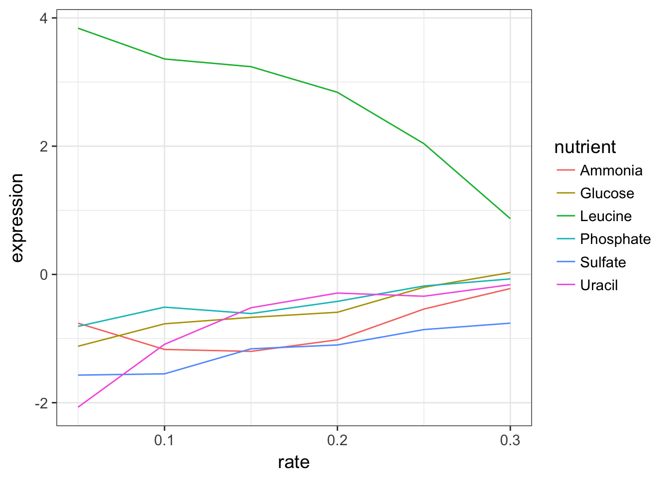

2.2 Plot the expression data of a biological process

For this, we don’t need to filter by single gene names as the raw data provides us some information on the biological process for each gene.
Extract all the genes in the leucine biosynthesis process and plot the expression in function of the growth rate for each nutrient.

Solution

cleaned_data_melt %>%
  filter(BP == "leucine biosynthesis") %>%
  ggplot(aes(x = rate, y = expression, colour = nutrient)) +
  geom_line() +
  facet_wrap(~ name)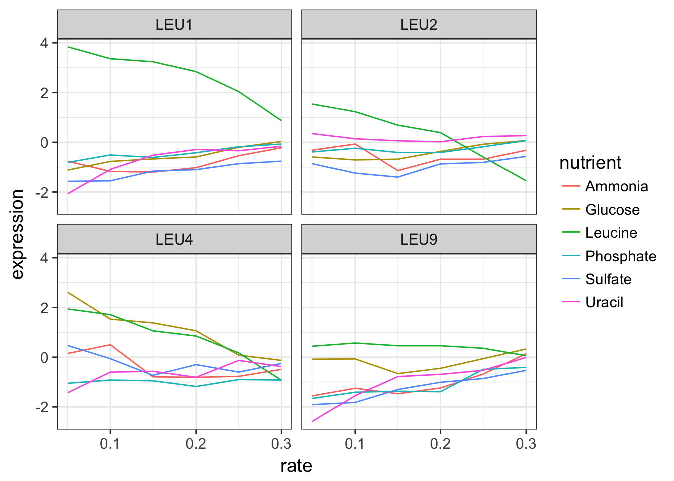

2.3 Perform a linear regression in top of the plots

Let’s play with the graph a little more. These trends look vaguely linear.
Add a linear regression with the appropriate ggplot2 function and carrefully adjust the method argument.

Solution

cleaned_data_melt %>%
  filter(BP == "leucine biosynthesis") %>%
  ggplot(aes(x = rate, y = expression, colour = nutrient)) +
  geom_point() +
  geom_smooth(method = "lm", se = FALSE) +
  facet_wrap(~ name)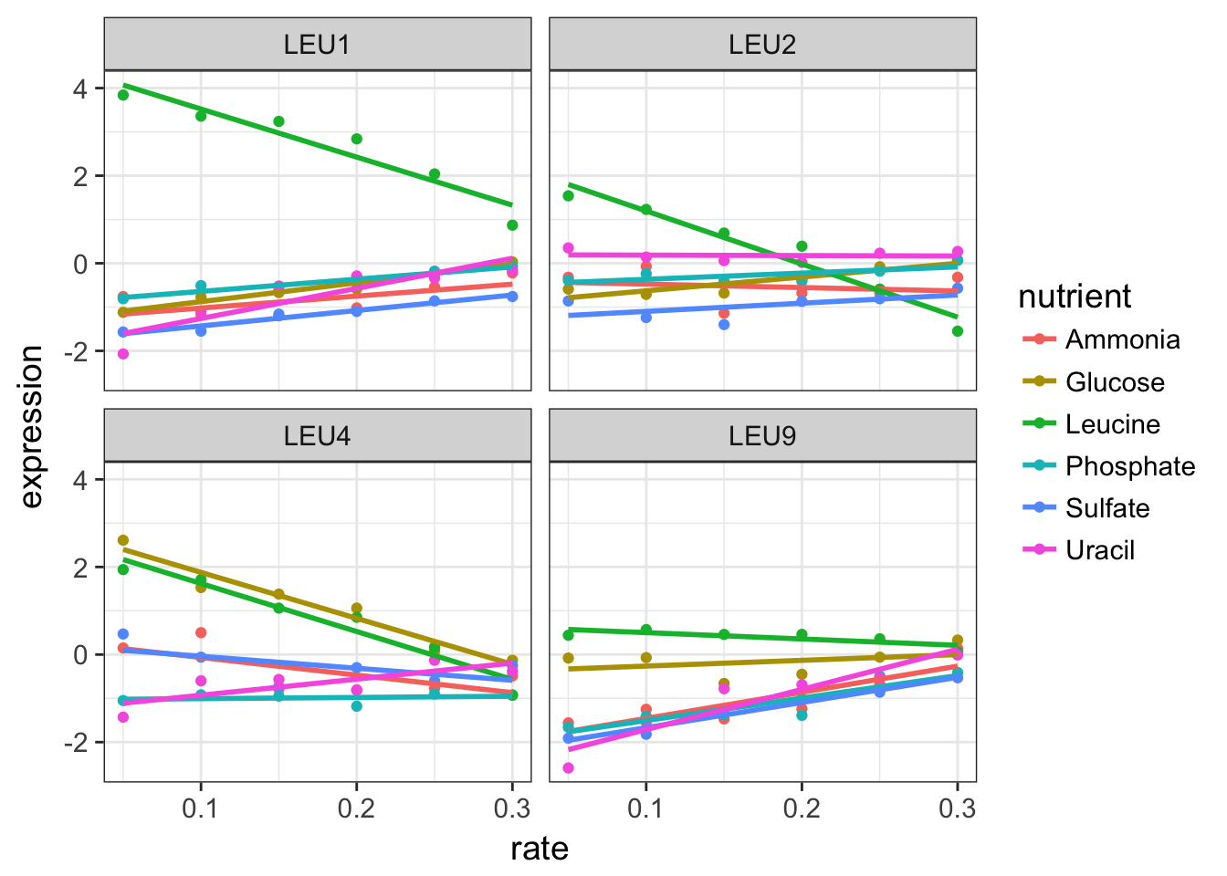

2.4 Switch to another biological process

Once the dataset is tidy, it is very easy to switch to another biological process. Instead of the “leucine biosynthesis”, plot the data corresponding to sulfur metabolism.

Tip

you can combine the facet headers using + in facet_wrap(). Adding the systematic name allows to get a name when the gene name is missing.

Solution

cleaned_data_melt %>%
  filter(BP == "sulfur metabolism") %>%
  ggplot(aes(x = rate, y = expression, colour = nutrient)) +
  geom_point() +
  geom_smooth(method = "lm", se = FALSE) +
  facet_wrap(~ name + systematic_name, scales = "free_y") # add 2 headers to facets with '+'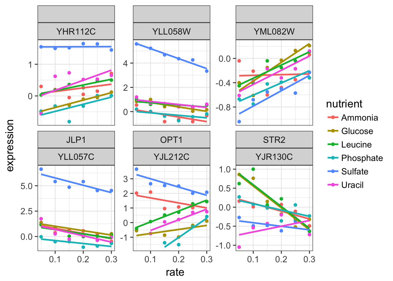

3. Linear models

We can see that most genes follow a linear trend under a starvation stress. Instead of manipulating all data points, we would like to estimate just the 2 parameters of a linear model. What are they? And what do they represent for this experiment?

Solution

Intercept, the value of gene expression for the maximum starvation
slope, the estimate of how the the gene expression varies in function of the starvation. A negative slope indicates that the gene is less expressed when starvation is relaxed

3.1 Perform all linear models

Perform a linear regression of expression explained by rate for all group of name, systematic_name and nutrient. By sure to convert the linear models to a tibble using broom as saved as cleaned_lm

The computation takes ~ 60 sec on my macbook pro. For test purposes, you may want to subsample per group a small number of genes

Solution

cleaned_data_melt %>%
  group_by(name, systematic_name, nutrient) %>%
  do(tidy(lm(expression ~ rate, data = .))) -> cleaned_lm

## Warning in summary.lm(x): essentially perfect fit: summary may be
## unreliable

How many models did you perform?

Solution

# divide by 2 since we have 2 coef per model
nrow(cleaned_lm) / 2

## [1] 33214

bonus question: you have observed a warning essentially perfect fit: summary may be unreliable, why? How can we clean up the dataset to avoid it?

Solution

# it is due to missing data where we have less than 6 points, which is already small to perform a linear model
# we can keep only groups where all 6 data points are presents
cleaned_data_melt %>%
  group_by(name, systematic_name, nutrient) %>%
  mutate(n = n()) %>%
  ggplot(aes(n)) + geom_histogram(bins = 40)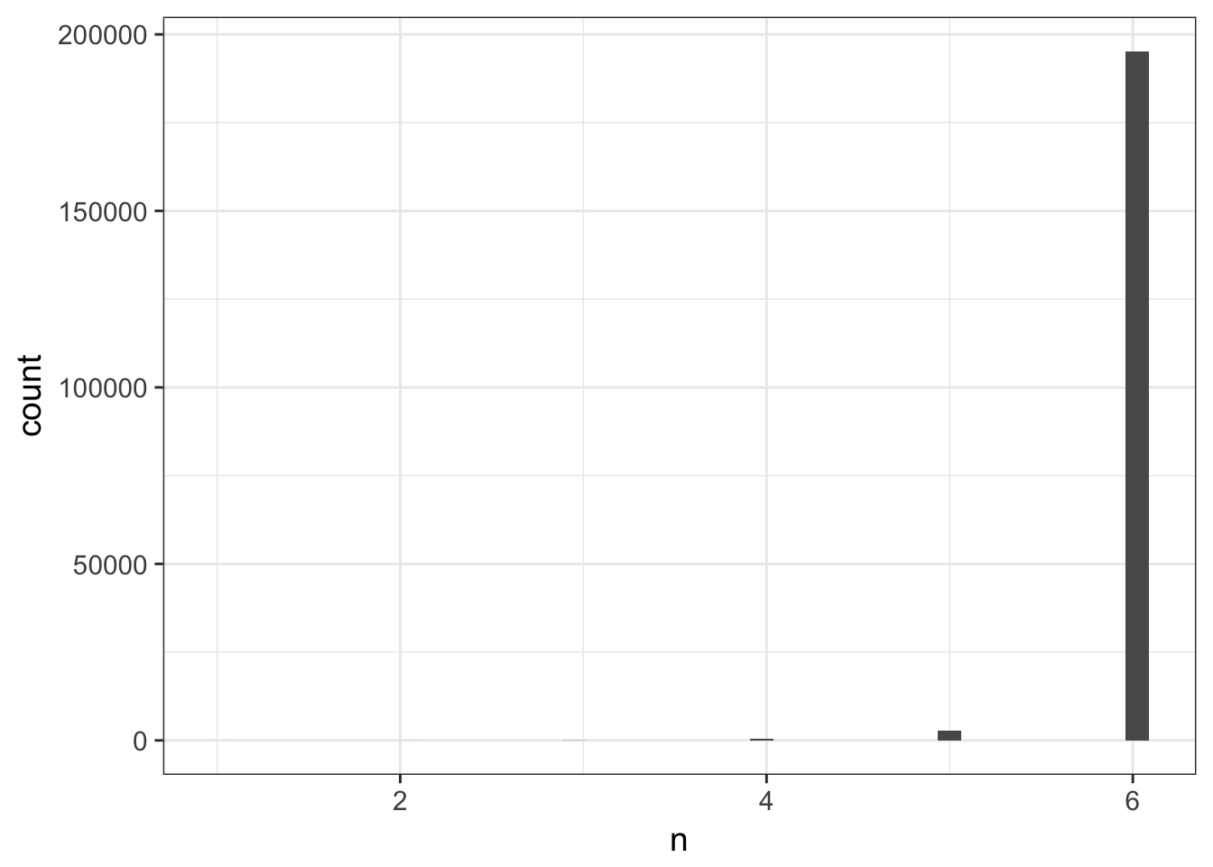

cleaned_data_melt %>%
  group_by(name, systematic_name, nutrient) %>%
  mutate(n = n()) %>%
  filter(n == 6) %>%
  do(tidy(lm(expression ~ rate, data = .))) -> cleaned_lm_clean

## Warning in summary.lm(x): essentially perfect fit: summary may be
## unreliable

3.2 Explore models, intercept values

For the gene LEU1, let’s look again at the linear models per nutrient and add as a dashed black line for mean of all intercepts.

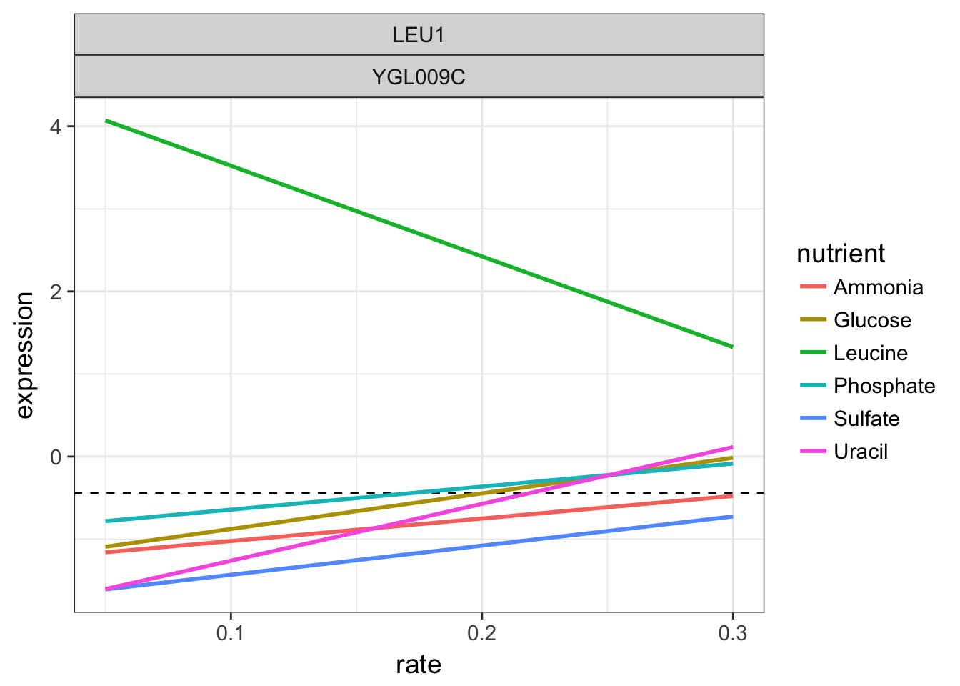
LEU1 linear models per nutrient

We can see that when leucine is the limiting factor, the yeast expresses massively this gene LEU1 to compensate. Remember that all experiments are performed at constant growth rates in this chemostat.

Now, compute the difference between the intercept and the mean(intercept) per systematic name, so for all nutrient per gene. And select the top 20 highest intercept values to their means. Save as top_20_intercept

Solution

cleaned_lm %>%
  filter(term == "(Intercept)") %>%
  group_by(systematic_name) %>%
  mutate(centered_intercept = estimate - mean(estimate)) %>%
  ungroup() %>%
  top_n(20, centered_intercept) -> top_20_intercept

merge those 20 genes with the cleaned_data_melt to retreived the original data points
plot the data points and linear trends for those top 20 genes. Instead of the systematic name in the header, use the molecular function (MF)

Solution

top_20_intercept %>%
  inner_join(cleaned_data_melt, by = c("systematic_name")) %>%
  ggplot(aes(x = rate, y = expression, colour = nutrient.y)) + 
  geom_hline(aes(yintercept = mean(expression)), linetype = "dashed") +
  geom_point() +
  geom_smooth(method = "lm", se = FALSE) +
  facet_wrap(~ name.y + MF)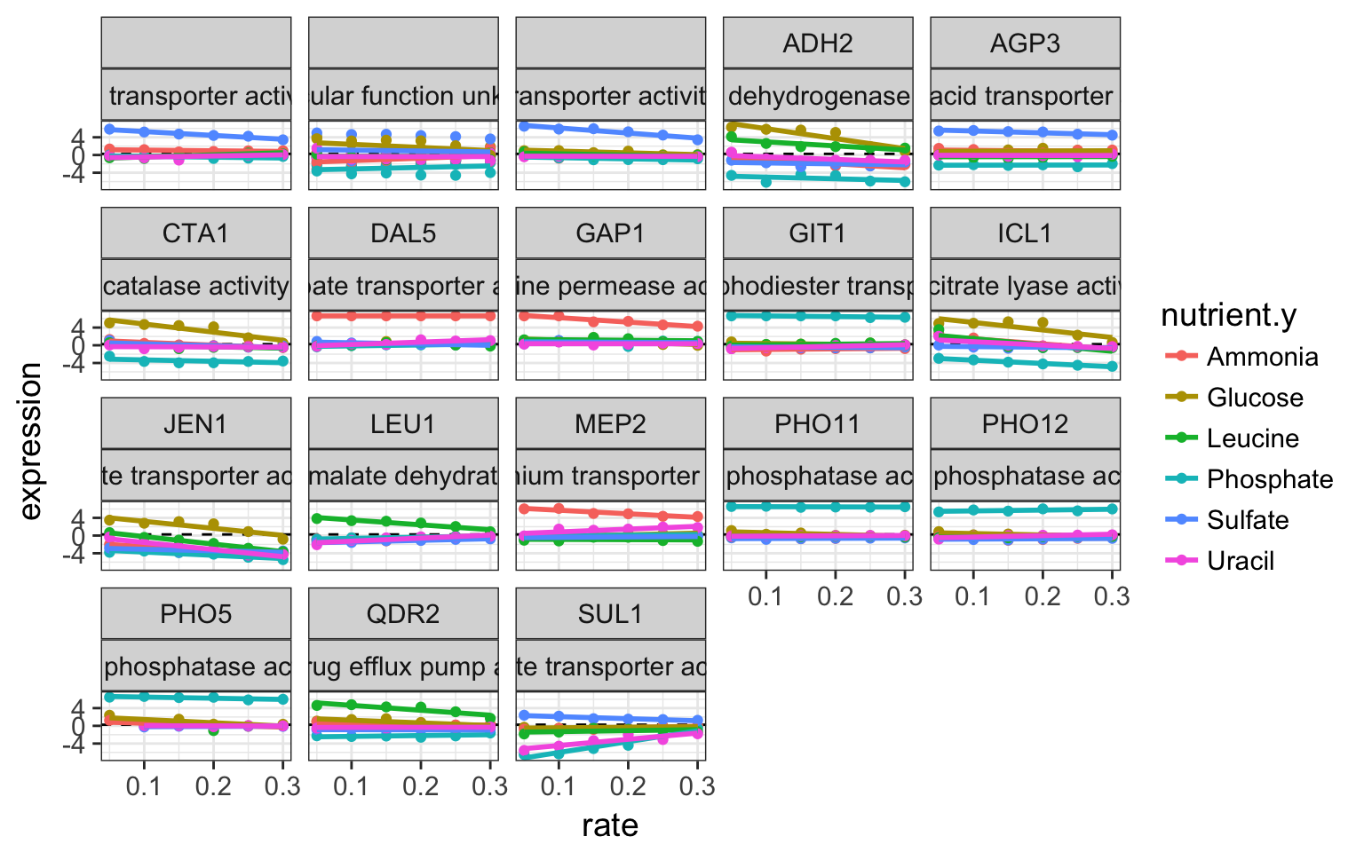

over expressed genes in starving conditions

what can conclude?

Solution

It is striking to see that most of genes have a transporter role. And like most higlhy expressed genes under high starvation like PHO genes are under phosphate starvation. The yeast is producing the necessary transporter to feed itself when the necessary metabolite is missing

3.3 Explore models, slope estimates

We can now have a look at the slope estimates.

first, filter the term for slope estimate rate and remove p-value that are missing. Save as rate_slopes

Solution

cleaned_lm %>%
  ungroup() %>%
  filter(term == "rate", !is.na(p.value)) -> rate_slopes

display the p-values histograms per nutrient

Solution

rate_slopes %>%
  ggplot(aes(x = p.value)) +
  geom_histogram(bins = 30) +
  facet_wrap(~nutrient)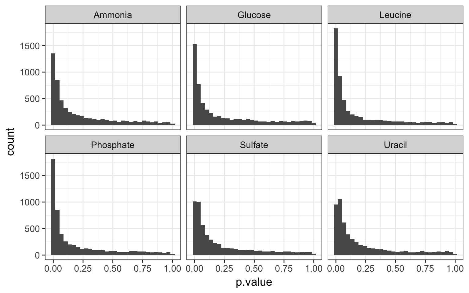

p values per nutrient

looking at those histograms, how do you estimate the ratio of null and alternative hypotheses?

Solution

close to the 0, this is where our alternative hypotheses lie. The p-values for the null follows a null distribution

how can retrieved the genes that belong most probably to the _alternative hypothesis?

Solution

we have perform 32000 tests, we must correct for multiple testing otherwise the false positives would be too high. We can compute the q-values

Solution

# see https://bioconductor.org/packages/release/bioc/html/qvalue.html
# for installation instructions
library(qvalue) 
rate_slopes %>%
  mutate(q.value = qvalue(p.value)$qvalues) -> rate_slopes

display the histograms of both p and q values per nutrient

Solution

rate_slopes %>%
  gather(prob, value, ends_with("value")) %>%
  ggplot(aes(x = value, fill = prob)) +
  geom_histogram(bins = 30, position = "dodge") +
  facet_wrap(~nutrient)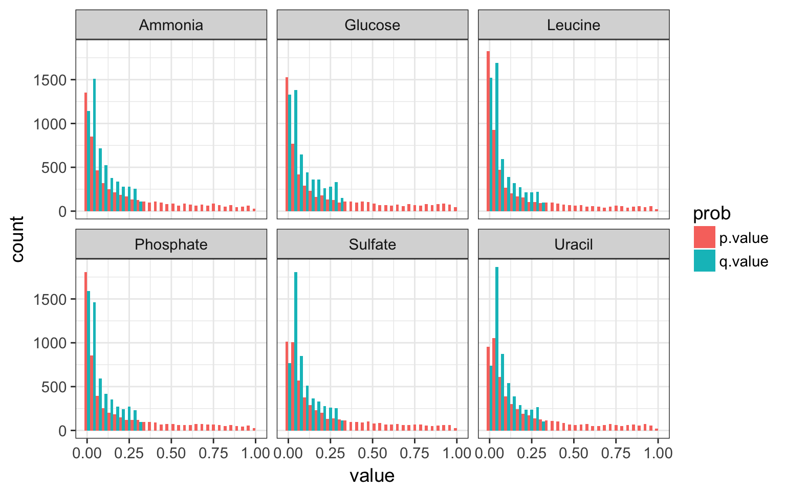

p and q values per nutrient

practical broom

Yeast dataset

Aurelien Ginolhac, Eric Koncina

4 May 2017

Project - set-up

Solution

1 Tidying the data

Solution

1.1 Many variables are stored in one column

Tip

Solution

Solution

Solution

Solution

1.2 Column headers are values, not variable names

Solution

Solution

Tip

Solution

1.3 Turn nutrient letters into more comprehensive words

Solution

1.4 Cleaning up missing data

Solution

2 Representing the data

2.1 Plot the expression data of the LEU1 gene

Solution

2.2 Plot the expression data of a biological process

Solution

2.3 Perform a linear regression in top of the plots

Solution

2.4 Switch to another biological process

Tip

Solution

3. Linear models

Solution

3.1 Perform all linear models

Solution

Solution

Solution

3.2 Explore models, intercept values

Solution

Solution

Solution

3.3 Explore models, slope estimates

Solution

Solution

Solution

Solution

Solution

Solution