R workshop

3^rd June 2016

R workshop

Day 2 - advanced

Modern R

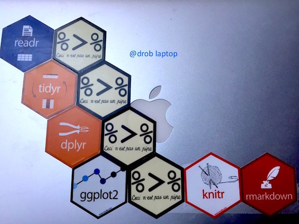
David Robinson summarized the goal on his laptop

see also what Karl Broman is recommanding for people who learnt R a while ago

Modern pipeline

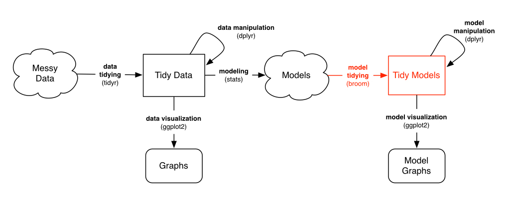
source: David Robinson check out David's broom presentation

reading data

Hadley Wickham and Wes McKinney recently released feather, a new python / R project.

It rapidly stores dataframes as binary files and preserves column types.

Managing multiple models

Tutorial based on the great conference by Hadley Wickham

purrr::map / dplyr::do

progress bar will be added

Functional programming and nested data_frames

Using purrr and tidyr. Hadley is focusing on every part of R to clean it up.

purrr revisits the apply family in a consistent way. tidyr::nest nests list in tibble::data_frame to keep related things together.

For loops emphasise on objects and not actions

compare (notice seq_along instead of 1:length(mtcars))

means <- vector("double", ncol(mtcars))
for (i in seq_along(mtcars)) {
  means[i] <- mean(mtcars[[i]])
}
means

##  [1]  20.090625   6.187500 230.721875 146.687500   3.596563   3.217250
##  [7]  17.848750   0.437500   0.406250   3.687500   2.812500

and

library("purrr")
map_dbl(mtcars, mean)

##        mpg        cyl       disp         hp       drat         wt 
##  20.090625   6.187500 230.721875 146.687500   3.596563   3.217250 
##       qsec         vs         am       gear       carb 
##  17.848750   0.437500   0.406250   3.687500   2.812500

Nested map

library("purrr")
library("dplyr", warn.conflicts = FALSE)
funs <- list(mean = mean, median = median, sd = sd)
funs %>%
  map(~ mtcars %>% map_dbl(.x))

## $mean
##        mpg        cyl       disp         hp       drat         wt 
##  20.090625   6.187500 230.721875 146.687500   3.596563   3.217250 
##       qsec         vs         am       gear       carb 
##  17.848750   0.437500   0.406250   3.687500   2.812500 
## 
## $median
##     mpg     cyl    disp      hp    drat      wt    qsec      vs      am 
##  19.200   6.000 196.300 123.000   3.695   3.325  17.710   0.000   0.000 
##    gear    carb 
##   4.000   2.000 
## 
## $sd
##         mpg         cyl        disp          hp        drat          wt 
##   6.0269481   1.7859216 123.9386938  68.5628685   0.5346787   0.9784574 
##        qsec          vs          am        gear        carb 
##   1.7869432   0.5040161   0.4989909   0.7378041   1.6152000

Keep related things together

Linear model per country

library("gapminder")
library("tidyr")
by_country_lm <- gapminder %>%
  mutate(year1950 = year - 1950) %>%
  group_by(continent, country) %>%
  nest() %>%
  mutate(model = map(data, ~ lm(lifeExp ~ year1950, data = .x)))
by_country_lm

## Source: local data frame [142 x 4]
## 
##    continent     country            data   model
##       (fctr)      (fctr)           (chr)   (chr)
## 1       Asia Afghanistan <tbl_df [12,5]> <S3:lm>
## 2     Europe     Albania <tbl_df [12,5]> <S3:lm>
## 3     Africa     Algeria <tbl_df [12,5]> <S3:lm>
## 4     Africa      Angola <tbl_df [12,5]> <S3:lm>
## 5   Americas   Argentina <tbl_df [12,5]> <S3:lm>
## 6    Oceania   Australia <tbl_df [12,5]> <S3:lm>
## 7     Europe     Austria <tbl_df [12,5]> <S3:lm>
## 8       Asia     Bahrain <tbl_df [12,5]> <S3:lm>
## 9       Asia  Bangladesh <tbl_df [12,5]> <S3:lm>
## 10    Europe     Belgium <tbl_df [12,5]> <S3:lm>
## ..       ...         ...             ...     ...

broom cleanup

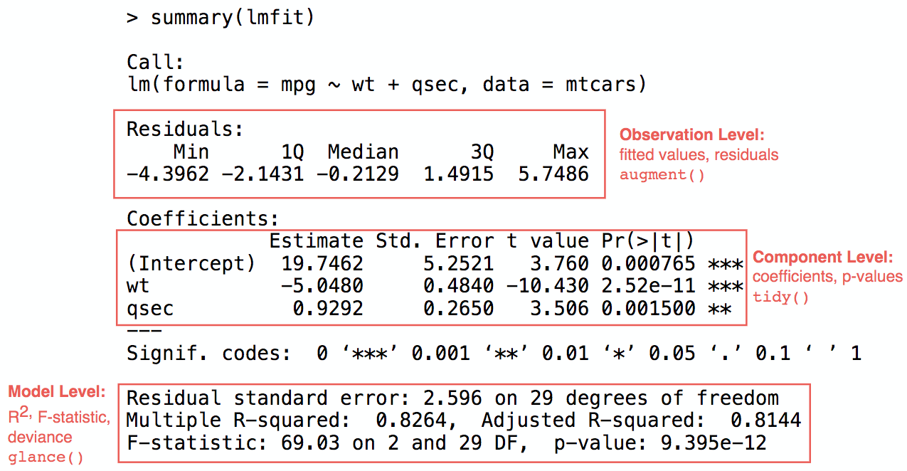
Tidying model coefficients

Use broom to extract, as neat data frames out of lm():

coefficients estimates: slope and intercept
\(r^2\)
residuals

library("broom")
models <- by_country_lm %>%
  mutate(glance  = map(model, glance),
         rsq     = glance %>% map_dbl("r.squared"),
         tidy    = map(model, tidy),
         augment = map(model, augment))
models

## Source: local data frame [142 x 8]
## 
##    continent     country            data   model              glance
##       (fctr)      (fctr)           (chr)   (chr)               (chr)
## 1       Asia Afghanistan <tbl_df [12,5]> <S3:lm> <data.frame [1,11]>
## 2     Europe     Albania <tbl_df [12,5]> <S3:lm> <data.frame [1,11]>
## 3     Africa     Algeria <tbl_df [12,5]> <S3:lm> <data.frame [1,11]>
## 4     Africa      Angola <tbl_df [12,5]> <S3:lm> <data.frame [1,11]>
## 5   Americas   Argentina <tbl_df [12,5]> <S3:lm> <data.frame [1,11]>
## 6    Oceania   Australia <tbl_df [12,5]> <S3:lm> <data.frame [1,11]>
## 7     Europe     Austria <tbl_df [12,5]> <S3:lm> <data.frame [1,11]>
## 8       Asia     Bahrain <tbl_df [12,5]> <S3:lm> <data.frame [1,11]>
## 9       Asia  Bangladesh <tbl_df [12,5]> <S3:lm> <data.frame [1,11]>
## 10    Europe     Belgium <tbl_df [12,5]> <S3:lm> <data.frame [1,11]>
## ..       ...         ...             ...     ...                 ...
## Variables not shown: rsq (dbl), tidy (chr), augment (chr)

Exploratory plots

Does linear models fit all countries?

library("ggplot2")
theme_set(theme_bw(14))
models %>%
  ggplot(aes(x = rsq, y = reorder(country, rsq)))+
  geom_point(aes(colour = continent))+
  theme(axis.text.y = element_text(size = 6))

focus on non-linear trends

models %>%
  filter(rsq < 0.55) %>%
  unnest(data) %>%
  ggplot(aes(x = year, y = lifeExp))+
  geom_line(aes(colour = continent))+
  facet_wrap(~ country)

shiny - code

library("shiny")
inputPanel(
  selectInput("country", "Select Country", levels(models$country))
)
output$rsq <- renderPlot({
  models %>%
  filter(country == input$country) %>%
  unnest(data) %>%
  ggplot(aes(x = year, y = lifeExp))+
  geom_line(aes(colour = continent))
})
renderUI({
 plotOutput("rsq", height = "400", width = "600")
})

shiny

library("shiny")
inputPanel(
  selectInput("country", "Select Country", levels(models$country))
)
output$country <- renderPlot({
  models %>%
  filter(country == input$country) %>%
  unnest(data) %>%
  ggplot(aes(x = year, y = lifeExp))+
  geom_line(aes(colour = continent))
})
renderUI({
 plotOutput("country", height = "400", width = "600")
})

shiny - rsquare

library("shiny")
inputPanel(
  sliderInput("rsq", "Select rsquared", min = 0, max = 1, 
              value = c(0, 0.2), dragRange = TRUE)
)
output$rsq <- renderPlot({
  models %>%
  filter(rsq >= input$rsq[1], rsq <= input$rsq[2]) %>%
  unnest(data) %>%
  ggplot(aes(x = year, y = lifeExp))+
  geom_line(aes(colour = continent))+
  facet_wrap(~ country)
})
renderUI({
 plotOutput("rsq", height = "400", width = "600")
})

All in all

models %>%
  unnest(tidy) %>%
  select(continent, country, rsq, term, estimate) %>%
  #filter(continent != "Africa") %>%
  spread(term, estimate) %>%
  ggplot(aes(x = `(Intercept)`, y = year1950))+
  geom_point(aes(colour = continent, size = rsq))+
  geom_smooth(se = FALSE)+
  scale_size_area()+
  labs(x = "Life expectancy (1950)",
       y = "Yearly improvement")

Error handling

purrr proposes safely() and possibly() to enable error-handling.

safely() is a type-stable version of try. It always returns a list of two elements, the result and the error, and one will always be NULL.

safely(log)(10)

## $result
## [1] 2.302585
## 
## $error
## NULL

safely(log)("a")

## $result
## NULL
## 
## $error
## <simpleError in .f(...): non-numeric argument to mathematical function>

to be investigated

Acknowledgments

Hadley Wickham
Robert Rudis
Ian Lyttle
David Robinson
Eric Koncina

R workshop

Day 2 - advanced

Modern R

Modern pipeline

reading data

Managing multiple models

purrr::map / dplyr::do

Functional programming and nested data_frames

For loops emphasise on objects and not actions

Nested map

Keep related things together

broom cleanup

Tidying model coefficients

Exploratory plots

Does linear models fit all countries?

focus on non-linear trends

shiny - code

shiny

shiny - rsquare

All in all

Error handling

Recommended reading

Acknowledgments