2nd June 2016
R workshop
Day 1 - beginner
Why learn R?
- Free!
- Packages
- Community
#rstatson twitter- rbloggers
- stackoverflow with a lot of tags like
dplyr,ggplot2etc

Packages
- CRAN reliable: package is checked during submit process

# install.packages("devtools")
devtools::install_github("hadley/readr")
- bioconductor. Check status
source("https://bioconductor.org/biocLite.R")
biocLite("limma")

More and more packages
Pipeline goal
David Robinson summarized the workflow on his laptop
Period of much suckiness
Period of much suckiness
Whenever you’re learning a new tool, for a long time you’re going to suck… But the good news is that it's typical, that’s something that happens to everyone, and it’s only temporary. – Hadley Wickham
R data structures
1 dimension: atomic vector
all elements of an atomic vector must be the same type source
concatenate elements of same type
x <- c(1, 1.24, "6")
x
## [1] "1"    "1.24" "6"
is.vector(x)
## [1] TRUE
x[1] # access 1st element
## [1] "1"
See if we enter 6 as character
x <- c(1, 1.24, "6")
x
## [1] "1"    "1.24" "6"
is.vector(x)
## [1] TRUE
is.list(x)
## [1] FALSE
is.atomic(x)
## [1] TRUE
1 dimension, lists
Lists are objects that could contain anything
l <- list(a = 1:3, b = c("hello", "bye"), data = head(iris, 2))
is.vector(l)
## [1] TRUE
is.list(l)
## [1] TRUE
is.atomic(l)
## [1] FALSE
l[1]
## $a
## [1] 1 2 3
l[[1]]
## [1] 1 2 3
# str(l)
subsetting
vector
x
## [1] "1"    "1.24" "6"
x[1]
## [1] "1"
x[-2] # return 1st and 3rd elements
## [1] "1" "6"
x[c(1, 3)] # return 1st and 3rd elements
## [1] "1" "6"
list
l[2]      # return a list
## $b
## [1] "hello" "bye"
l[2][1]   # makes no sense
## $b
## [1] "hello" "bye"
l[[2]]    # return a vector
## [1] "hello" "bye"
l[[2]][1] # return 1st element, 2nd atomic vector
## [1] "hello"
factor
f <- rep(c("Male", "Female"), each = 4)
f
## [1] "Male"   "Male"   "Male"   "Male"   "Female" "Female" "Female" "Female"
ff <- factor(f)
ff # levels are like dictionnary keys
## [1] Male   Male   Male   Male   Female Female Female Female
## Levels: Female Male
str(ff) # structure of factor, integer behind
##  Factor w/ 2 levels "Female","Male": 2 2 2 2 1 1 1 1
table(ff) # useful command to count entities
## ff
## Female   Male
##      4      4
ff[3] <- "t" # error! "t" not in levels
## Warning in `[<-.factor`(`*tmp*`, 3, value = "t"): invalid factor level, NA
## generated
Accessing lists' elements
2 dimensions: homogenous elements
matrix
matrix(data = 1:6, nrow = 2, ncol = 3)
##      [,1] [,2] [,3]
## [1,]    1    3    5
## [2,]    2    4    6
2 dimensions: data frames
which are lists where all columns have equal length
class(iris)
## [1] "data.frame"
class(unclass(iris))
## [1] "list"
Actually, better to use tbl_df tibble diff rstudio blog
data_frame() does much less than data.frame():
- never changes the type of the inputs (e.g. it never converts strings to factors!)
- never changes the names of variables
- never creates row.names()
- never print ALL rows
but display
- column types
- groups (
dplyr::group_by())
subsetting data frames
data frame are lists
mtcars[[1]]
##  [1] 21.0 21.0 22.8 21.4 18.7 18.1 14.3 24.4 22.8 19.2 17.8 16.4 17.3 15.2
## [15] 10.4 10.4 14.7 32.4 30.4 33.9 21.5 15.5 15.2 13.3 19.2 27.3 26.0 30.4
## [29] 15.8 19.7 15.0 21.4
mtcars[["mpg"]]
##  [1] 21.0 21.0 22.8 21.4 18.7 18.1 14.3 24.4 22.8 19.2 17.8 16.4 17.3 15.2
## [15] 10.4 10.4 14.7 32.4 30.4 33.9 21.5 15.5 15.2 13.3 19.2 27.3 26.0 30.4
## [29] 15.8 19.7 15.0 21.4
but $ is a shorthand for [[
mtcars$mpg
##  [1] 21.0 21.0 22.8 21.4 18.7 18.1 14.3 24.4 22.8 19.2 17.8 16.4 17.3 15.2
## [15] 10.4 10.4 14.7 32.4 30.4 33.9 21.5 15.5 15.2 13.3 19.2 27.3 26.0 30.4
## [29] 15.8 19.7 15.0 21.4
Rstudio
Integrated Development Editor
Layout, 4 panels
Features
- Package management (including building)
- Console to run
R, with syntax highligther - Editor to work with scripts / markdown
- auto-completion using TAB
- Cheatsheets
- Keyboard shortcuts
Cmd + Enter (mac) orCtrl + Enter (PC): sends the line or selection from the editor to the console and runs it.
↑: in the console browse previous commands
Update options
Recommended in the r4ds To get a clean environment at start-up
Projects
Solve most issues with working directories, get rid of setwd()
Chaining
The pipe operator %>%
magrittr by Stefan Milton Bache
Compare:
set.seed(124)
x <- rnorm(10)
mean(x)
## [1] 0.2147669
round(mean(x), 3)
## [1] 0.215
with:
set.seed(124)
rnorm(10) %>% mean %>% round(3)
## [1] 0.215
Easier to read
natural from left to right.
Even better with one instruction per line and indentation
set.seed(124)
rnorm(10) %>%
  mean %>%
  round(3)
## [1] 0.215
placeholder = .
x %>% f(.)
#stands for (pipe to the 1st function argument)
f(x)
When not 1st argument
sub("b", "B", letters[1:3])
## [1] "a" "B" "c"
letters[1:3] %>% sub("b", "B") # raises warning!
## Warning in sub(., "b", "B"): argument 'pattern' has length > 1 and only the
## first element will be used
## [1] "B"
letters[1:3] %>% sub("b", "B", .)
## [1] "a" "B" "c"
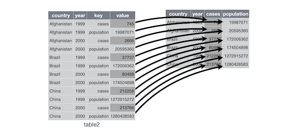
Tidying data
tidyr
Definitions
- Variable: A quantity, quality, or property that you can measure.
- Observation: A set of values that display the relationship between variables. To be an observation, values need to be measured under similar conditions, usually measured on the same observational unit at the same time.
- Value: The state of a variable that you observe when you measure it.
Rules
- Each variable is in its own column
- Each observation is in its own row
- Each value is in its own cell

Convert Long / wide format
The wide format is generally untidy but found in the majority of datasets


Demo with the iris dataset
head(iris, 3)
##   Sepal.Length Sepal.Width Petal.Length Petal.Width Species
## 1          5.1         3.5          1.4         0.2  setosa
## 2          4.9         3.0          1.4         0.2  setosa
## 3          4.7         3.2          1.3         0.2  setosa
gather
library("tidyr")
iris_melt <- iris %>%
  tibble::rownames_to_column() %>%
  dplyr::tbl_df() %>%
  gather(flower, measure, contains("al"))
iris_melt
## Source: local data frame [600 x 4]
##
##    rowname Species       flower measure
##      <chr>  <fctr>        <chr>   <dbl>
## 1        1  setosa Sepal.Length     5.1
## 2        2  setosa Sepal.Length     4.9
## 3        3  setosa Sepal.Length     4.7
## 4        4  setosa Sepal.Length     4.6
## 5        5  setosa Sepal.Length     5.0
## 6        6  setosa Sepal.Length     5.4
## 7        7  setosa Sepal.Length     4.6
## 8        8  setosa Sepal.Length     5.0
## 9        9  setosa Sepal.Length     4.4
## 10      10  setosa Sepal.Length     4.9
## ..     ...     ...          ...     ...
spread
iris_melt %>%
  spread(flower, measure)
## Source: local data frame [150 x 6]
##
##    rowname    Species Petal.Length Petal.Width Sepal.Length Sepal.Width
##      <chr>     <fctr>        <dbl>       <dbl>        <dbl>       <dbl>
## 1        1     setosa          1.4         0.2          5.1         3.5
## 2       10     setosa          1.5         0.1          4.9         3.1
## 3      100 versicolor          4.1         1.3          5.7         2.8
## 4      101  virginica          6.0         2.5          6.3         3.3
## 5      102  virginica          5.1         1.9          5.8         2.7
## 6      103  virginica          5.9         2.1          7.1         3.0
## 7      104  virginica          5.6         1.8          6.3         2.9
## 8      105  virginica          5.8         2.2          6.5         3.0
## 9      106  virginica          6.6         2.1          7.6         3.0
## 10     107  virginica          4.5         1.7          4.9         2.5
## ..     ...        ...          ...         ...          ...         ...
Separate / Unite
unite
df %>%
  unite(date, c(year, month, day), sep = "-") -> df_unite
separate, use quotes since we are not refering to objects
df_unite %>%
  separate(date, c("year", "month", "day"))
## Source: local data frame [3 x 4]
##
##    year month   day value
##   <chr> <chr> <chr> <chr>
## 1  2015    11    23  high
## 2  2014     2     1   low
## 3  2014     4    30   low
Help
using ? or help()
?gather
or using the Help tab next to the Packages tab.
Reading data
readr
read_tsv
Guess column types and give warnings.
library("readr")
soft <- read_tsv("data/GDS5079.soft", skip = 42, na = "null")
## Warning: 2 parsing failures.
##   row      col   expected             actual
## 35557 10344614 an integer !dataset_table_end
## 35557 NA       6 columns  1 columns
Viewer utility
View(soft)
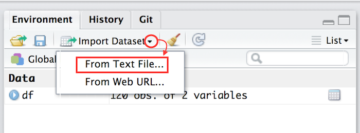
Easier: import file utility
Using Rstudio, right top panel. Select directly your file. This actually uses readr.

Plotting
ggplot2
Why tidy is useful?
library("tidyr")
library("ggplot2")
iris %>%
  gather(flower, measure, 1:4) %>%
  ggplot()+
  geom_boxplot(aes(x = Species, y = measure, fill = flower))
Scatterplots
iris %>%
  ggplot(aes(x = Sepal.Length, y = Sepal.Width, colour = Species))+
  geom_point()+
  geom_smooth(method = "lm", se = FALSE)+
  xlab("Length")+
  ylab("Width")+
  ggtitle("Sepal")
More aesthetics
iris %>%
  ggplot(aes(x = Sepal.Length, y = Sepal.Width,
             size = Petal.Length / Petal.Width,
             colour = Species))+
  geom_point()+
  scale_size_area("Petal ratio Length / Width")+
  #scale_colour_brewer(palette = 1, type = "qual")+
  scale_colour_manual(values = c("blue", "red", "orange"))+
  xlab("Sepal.Length")+
  ylab("Sepal.Width")
in / out aesthetics
iris %>%
  ggplot(aes(x = Sepal.Length, y = Sepal.Width))+
  geom_point(aes(colour = Species))
iris %>%
  ggplot(aes(x = Sepal.Length, y = Sepal.Width))+
  geom_point(aes(colour = "Species"))
in / out aesthetics
iris %>%
  ggplot(aes(x = Sepal.Length, y = Sepal.Width))+
  geom_point(colour = "Species") # Error
iris %>%
  ggplot(aes(x = Sepal.Length, y = Sepal.Width))+
  geom_point(colour = "red")
histogram
iris_melt %>%
  ggplot()+
  geom_histogram(aes(x = measure, fill = flower))
## `stat_bin()` using `bins = 30`. Pick better value with `binwidth`.
Barplots - stack
by default, geom_bar counts. For mapping values use stat = "identity"
iris_melt %>%
  ggplot()+
  geom_bar(aes(x = Species, y = measure, fill = flower), stat = "identity")
iris_melt %>%
  ggplot()+
  geom_bar(aes(x = measure, fill = flower))
Barplots - relative
iris_melt %>%
  ggplot()+
  geom_bar(aes(x = Species, y = measure, fill = flower), position = "fill", stat = "identity")
Barplots - dodge
iris_melt %>%
  ggplot()+
  geom_bar(aes(x = Species, y = measure, fill = flower), position = "dodge", stat = "identity")
heatmap
iris_melt %>%
  ggplot()+
  geom_tile(aes(x = Species, y = flower, fill = measure))+
  scale_fill_gradient(low = "yellow", high = "red", limits = c(0, 8))
Density and faceting
transparency using the alpha parameter
iris_melt %>%
  ggplot()+
  geom_density(aes(x = measure, fill = Species, colour = Species), alpha = 0.6)+
  facet_wrap(~ flower, scale = "free")+
  theme_bw()
facetting
transparency using the alpha parameter
iris_melt %>%
  ggplot()+
  geom_density(aes(x = measure, fill = Species, colour = Species), alpha = 0.6)+
  facet_grid(Species ~ flower, scale = "free")+
  theme_bw()
theme
Recommended reading
- data structures by Hadley
- R for data science by Hadley & Garrett
- reading data
- tidy data
- plotting
- ggplot2 documentation by Hadley / Winston
- ggplot2 layer by layer by Hadley
- ggplot2 extensions by Daniel Emaasit
- Excellent ressource on
R(in French) Introduction to R by Ewen Gallic
Acknowledgments
- Hadley Wickham
- Garrett Grolemund
- Jenny Bryan
- Ewen Gallic
- David Robinson
- Eric Koncina
- Tony Heurtaux